All published articles of this journal are available on ScienceDirect.

A Reliable PSO-based ANN Approach for Predicting Unconfined Compressive Strength of Sandstones
Abstract
Background:
The reliable determination of geomechanical parameters of rocks such as Unconfined Compressive Strength (UCS) using laboratory methods is problematic and time-consuming. In this regard, the construction of reliable predictive models for assessing the UCS is of advantage.
Objective:
The main purpose of this work is to propose the use of a reliable PSO-based ANN approach for predicting the UCS of sandstones.
Methods:
For this purpose, laboratory tests were performed on 60 sandstone specimens. The laboratory tests comprise P-wave velocity, dry density, Schmidt hardness and UCS. Apart from the latter, the other laboratory tests were set as model inputs. Prediction performance of the constructed model was assessed according to the criteria including coefficient of determination (R2), Root Mean Squared Error (RMSE) and Variance Account For (VAF).
Results:
Results (R2= 0.974 and RMSE = 0.086 and VAF = 97.5) showed the reliability of the constructed PSO-based ANN model to predict UCS of sandstones.
Conclusion:
Hence, this study recommends utilizing PSO-based ANN as a feasible tool for assessing UCS of sandstones. Nevertheless, further research is suggested for model generalization purposes.
1. INTRODUCTION
Rock characterization plays an important role in design of geotechnical structures. There are several methods for determining the engineering properties of rocks. These methods are often divided into direct and indirect methods. Unconfined Compressive Strength (UCS) of rock is one of the direct methods for evaluating the compressive behavior of rock samples. The test is standardized by ISRM [1]. However, determining UCS is relatively costly and destructive. Additionally, sometimes providing high-quality rock specimens is a difficult task to be accomplished more especially in the case of porous, thinly bedded, foliated, weak and weathered rocks. These impeding factors encourage laboratory technicians to utilize easier methods (indirect methods) for assessing the compressing strength of rocks. Indirect methods including point load index text, Is(50), P-wave velocity test, Schmidt hammer test, to name a few, are relatively easier and quick. These index tests can be related to the UCS test. Many researchers recommend conventional regression-based equations for relating rock index tests to UCS. In this regard, Momeni et al. [2], in their review paper, provided a comprehensive list of these equations. In another study, Nazir et al. [3] proposed a relatively reliable correlation between UCS and Brazilian tensile strength of rocks. Nazir et al. [4] also recommended a correlation between UCS and Schmidt hammer rebound number (SRn). Sari [5] proposed two correlations between UCS and P-wave velocity test as well as UCS and Schmidt hammer rebound number. In the recent past, the application of artificial intelligence in geotechnical engineering is underlined in many studies [6-20]. Other researchers highlighted the feasibility of soft computing in solving civil Engineering problems [21-37]. Sometimes, to have a better evaluation, it is suggested to investigate the effect of a number of parameters on the parameter of interest. For example, although UCS can be estimated from BTS using conventional correlations, some studies suggest the prediction of UCS from multivariate equations. Nevertheless, in general, multivariate equations are not working well enough for non-linear problems when the contact nature between input and output parameters is unknown. Among different artificial intelligence techniques, many researchers suggested the feasibility of artificial neural networks in predicting the UCS of rocks [38]. However, as stated in the literature, ANN suffers from two major drawbacks [39]: slow rate of learning and getting trapped in local minima. Several studies reported the improvement of ANN by implementing the optimization algorithms including particle swarm optimization algorithm [40], genetic algorithm [41], and imperialist competitive algorithm [42] to name a few. This paper is aimed to predict UCS of sandstones using the PSO-based ANN model. Additionally, the Multiple Linear Regression (MLR) was used for estimating UCS. Although UCS prediction has drawn considerable attention in the literature, presenting new real datasets from different parts of world is always of interest as rock behavior is site specific varies from a place to another place.
2. LITERATURE REVIEW
Numerous correlations have been proposed for estimating UCS in the literature. In Table 1, the regression-based correlations are tabulated and Table 2 presents the proposed artificial intelligence-based predictive models of UCS. Among others, Meulenkamp and Grimma [43] developed a predictive model of UCS using ANN. The size of the dataset in their study was 194. They used Equotip value, porosity, density, and grain size as their input parameters. According to their conclusion, the coefficient of determination of their model was high enough (R2 = 0.94). In another study, Singh et al. [44] proposed an ANN-based predictive model of UCS based on 112 datasets. They used petrography data to train and test their model. Also, Dehghan et al. [45] recommended the feasibility of ANN in predicting UCS. They developed the model using 30 datasets. Their input data included Vp, point load index values, SRn, and porosity. They reported R2 = 0.86 and concluded that their predictive model is reliable enough. Rezaei et al. [46] developed a Fuzzy Inference System (FIS) to predict UCS of rocks based on 93 datasets . Their model input consisted of porosity, SRn and density. Monjezi et al. [47] used the same input parameters. However, Monjezi et al. utilized a GA-based ANN model for developing their model. The reliability of the predictive model of UCS proposed by Monjezi et al. in terms of R2 was 0.96. Using 72 datasets, Beiki et al. [48] developed a predictive model of UCS using genetic programming. The input parameters used in their study were density, porosity and Vp. They reported R2 equal to 0.94 as the performance index of their model. Yagiz et al. [49] utilized ANN for developing a predictive model of UCS using 54 datasets . Their input parameters were porosity, point load index value, dry unit weight, Vp, and SRn. However, according to their conclusion, their proposed model was not reliable enough (R2 = 0.50). Using 105 sets of data, Torabi-kaveh et al. [50] recommended an ANN-based predictive model of UCS. Their proposed model with R2 = 0.95 was highly reliable. Similar to the aforementioned works, they used density, porosity and Vp as the model inputs. Yesiloglu-Gultekin et al. [51] implemented an Adaptive Neuro-fuzzy Inference System (ANFIS) for UCS prediction. They used Brazilian tensile strength and Vp as the model inputs. The size of the dataset in their study was 75. The reported R2 in their study was 0.60. In another study, Abdi et al. [38] predicted the UCS of sedimentary rocks using ANN. In order to train their model, they collected 196 different types of rock specimens including limestone, conglomerate, sandstone, and marl. The input parameters of their suggested model were dry unit weight, Vp, porosity, and water absorption. The correlation coefficient, R, of their proposed model for testing data was 0.93. Overall, the aforementioned studies, as well as studies highlighted in Table 2, indicate the workability of artificial intelligence more especially artificial neural network in predicting UCS of rock using different rock engineering properties as well as rock index tests.
| Reference | Correlation | Reliability | Rock Type |
|---|---|---|---|
| Kahraman et al. [52] | UCS = 10.61BTS | R2 = 0.54 | Different rock types including limestone |
| Sari [5] | UCS = 4.969exp(0.058RL) | R2 = 0.575 | Different rock types |
| Sari [5] | UCS = 5.912VP1.741 | R2 = 0.645 | Different rock types |
| Altindag and Guney [53] | UCS = 12.38BTS1.0725 | R = 0.9 | Different rock types including limestone |
| Gokceoglu and Zorlu [54] | UCS = 6.8BTS +13.5 | R = 0.65 | - |
| Nazir et al. [3] | UCS = 9.25BTS0.947 | R2 = 0.90 | 20 Limestone samples |
| Karaman et al. [55] | UCS = 24.301+4.874BTS | R2 = 0.90 | 37 Rock samples including Basalt and limestone |
| Broch and Franklin [56] | UCS = 23.7 Is(50) | - | - |
| Bieniawski [57] | UCS = 23 Is(50) | - | Different type of rocks |
| Kahraman et al. [58] | UCS = 10.22 Is(50) + 24.31 | R2 = 0.75 | 38 Different rock samples |
| Basu and Aydin [59] | UCS = 18 Is(50) | R2 = 0.97 | 40 Granitic rock samples |
| Yilmaz and Yuksek [60] | UCS = 12.4 Is(50) - 9.0859 | R2 = 0.81 | 39 Sets of gypsum samples |
| Diamantis et al. [61] | UCS = 19.79 Is(50) | R2 = 0.74 | 32 Samples of serpentinite rock |
| Kahraman [62] | UCS = 14.68Is(50) − 8.67 | R = 0.88 | 32 Pyroclastic specimens |
| Sarkar et al. [63] | UCS=0.038Vp-50 | R2=0.93 | 13types of different rock |
| Kilic and Teymen [64] | UCS=0.0137RL2.2721 | R= 0.93 | Different rock types |
| Cobanoglu and Selik [65] | UCS=6.59 RL -212.6 | R= 0.65 | Limestone, sandstone, cement mortar |
| Tugrul and Zarif [66] | UCS=8.36 RL -416 | R= 0.87 | 19 Granite rock samples |
| Nazir et al. [4] | UCS=12.83 e(0.0487 RL) | R = 0.95 | 20 Limestone samples |
| Aydin and Basu [67] | UCS=1.4459e0.0706 RL | R = 0.92 | Granitic rocks |
| Gupta [68] | UCS=1.15 RL -15 | R = 0.95 | Granite |
| Sharma and Singh [69] | UCS = 0.0642VP – 117.99 | R2 = 0.90 | 49 samples in different rock types |
| Moradian and Behnia [70] | UCS=165.05e(- .452/Vp) | R2 = 0.7 | 64 different rock samples |
| Khandelwal [71] | UCS = 0.033 VP – 34.83 | R2 = 0.87 | 12 samples of a wide rock types |
| Diamantis et al. [61] | UCS=0.11 VP - 515.56 | R2 = 0.81 | 32 samples of serpentinite rock |
| Altindag [72] | UCS = 12.743 VP1.194 | R = 0.76 | 97 rock specimens (mainly limestone) |
| Cobanoglu and Celik [65] | UCS=56.71 VP - 192.93 | R2 = 0.67 | 150 core samples of different rocks |
| Xu et al. [73] | UCS=2.98 e(0.06 RL) | R = 0.95 | Mica-schist |
| Jamshidi et al. [74] | UCS=133.77 Ln Vp-1048 | R= 0.90 | Limestone |
| Entwisle et al. [75] | UCS= 0.78 e 0.88VP | R2 = 0.53 | 171 samples of Volcanic rock |
| Reference | Technique | Dataset Number | Input Layer | R2 |
|---|---|---|---|---|
| Verma and singh [76] | ANFIS | - | R, W, ρ, BTS, Vp | 0.763 |
| Singh et al. [77] | ANFIS | 85 | ρ, Is(50), WA | 0.664 |
| Rezaei et al. [78] | ANFIS | 93 | Rn, n, ρ | 0.97 |
| Saedi et al. [79] | ANFIS | 120 | CPI, Is(50), BTS, BPI | 0.854 |
| Rabbani et al. [80] | ANN | - | n, BD, Sw | 0.96 |
| Sharma et al. [81] | ANFIS | 94 | γd, Vp, SDI | 0.978 |
| Ceryan et al. [82] | ANN | 55 | n, Id, Vm, ne, PSV | 0.88 |
| Zorlu et al. [83] | ANN | 138 | q, pd, cc | 0.76 |
| Yilmaz and Yuksek [60] | ANFIS | 121 | Vp, Is(50), SRn, WC | 0.94 |
| Jahanbakhshi et al. [84] | ANN | 133 | ρ, n, Vp | 0.96 |
| Majidi and Rezaei [85] | ANN | 93 | R, Rn, n, ρ | 0.97 |
| Sarkar et al. [86] | ANN | 40 | Vp, Is(50), Id, ρ | 0.99 |
| Fang et al. [87] | ANN-GP-PSO-ICA | 71 | SRn,Vp, Is(50),n | - |
| Momeni et al. [40] | PSO-ANN | 66 | SRn,Vp, Is(50), ρ | 0.95 |
| Mishra and Basu [88] | FIS | 60 | Vp, Is(50), BPI, SRn | 0.98 |
| Tonnizam Mohamad et al. [39] | ANN-PSO | 40 | Is(50), BD, Vp, BTS | 0.97 |
| Jahed Armaghani et al. [89] | ANFIS | 45 | Vp, ρ, PSV | 0.98 |
| Jahed Armaghani et al. [42] | ICA-ANN | 71 | n, Vp, SRn, Is(50) | 0.92 |
| Tonnizam Mohamad et al. [90] | PSO-ANN | 38 | Id, d, Is(50),Vp,WC | 0.98 |
3. MATERIALS AND METHODS
3.1. Artificial Neural Network
Artificial Neural Network (ANN) can be seen as a black box which is utilized when there is a highly nonlinear relationship between input and output of a model. The term black box sometimes is given to the ANN because unlike regression-based techniques, there is no specific formula for estimating the parameter of interest. Multilayer Perceptron (MLP) is the most common type of ANNS for both estimation and classification problems [91-95]. The structure of the MLP network includes input, hidden and output layers. There is no specific approach for determining the number of hidden layers as well as the number of hidden nodes . However, almost in most civil engineering problems, the use of one hidden layer is good enough. It is due to the fact that in civil engineering problems, collecting experimental data for training the ANN-based predictive models is difficult. In other words, when the size of dataset is small, implementation of more than one hidden layer can increase the likelihood of the model overtraining and overfitting. Nevertheless, the input, hidden and output layers are connected to each other using hidden nodes or neurons. That is the input parameters are connected to hidden nodes in the hidden layer and the aforementioned hidden nodes are connected to the model output. Each connection has a weight. Depending on the training algorithm, the weight of each connection is determined. One of the most famous training algorithms is backpropagation technique. In this method, the network starts to feed forward. In the hidden layer, to have a hidden node output value, a transfer function is applied to the input values of each hidden node. The input value of each hidden nodes is simply determined by the summation of connection weights of that hidden node as well as a threshold value known as bias. This process is repeated between the hidden layer and the output layer and the value of the output parameter is predicted. The predicted output is compared with the target (already known) and the error is estimated. The network has to backpropagate and update its weights (if the error is not desirable). In the hybrid ANNs, instead of conventional methods, the weights are optimized using optimization algorithms. Detail of ANNs is out of the scope of this paper and readers are referred to other studies to get more detail [9].
3.2. Particle Swarm Optimization
Particle Swarm Optimization was originally proposed by Eberhart and Kennedy [96]. Several studies have been conducted on the efficiency of PSO in achieving optimal solutions in large search spaces, e.g., the study by Mendes et al. [97]. In this regard, a primary advantage of PSO is the simple evolutionary process that distinguishes it from other optimization algorithms. Victoire and Jeyakumar [98] showed that PSO is an effective computational tool that cuts the required amount of memory in comparison to other similar algorithms. PSO works with two simple equations.
 |
(1) |
 |
(2) |
In Eqs. 1 and 2, vnew, v, pnew, and p denote the new velocity, current velocity, new position, and current position, respectively, for a given particle among a set of particles. Also, C1 and C2 show acceleration constants; pbest indicates the best position of a particle and gbest stands for the best position of the particles in the set; r1 and r2 are arbitrary values in the range of 0 to 1. PSO optimization is initiated by randomly selecting some particles. In the current context, it starts with initializing the ANN weights. A random velocity and position are assigned to each particle (i.e., ANN weight). Next, an iterative process is employed to seek the optimum solution by recording the Pbest and gbest values of each particle during each interaction. Afterward, using Eqs. 1 and 2, the changes in the positions of the particles with respect to their experiences and the position of the other particles are determined [99]. These positions are updated until reaching a predefined “termination criterion” or the optimum solution [100].
3.3. PSO-based ANN
To enhance the efficiency of ANNs, often optimization algorithms like PSO are implemented. This is generally attributed to the shortcomings of ANNs in getting trapped in local minima. The problem can be solved if ANN is coupled with global search algorithms like PSO. The PSO component of such a hybrid system enables it to find a global minimum while searching. Accordingly, a hybrid PSO-based ANN model enjoys the benefits of both PSO and ANN; PSO searches for the entire minima in the search space and ANN then employs them to obtain the best solution. It is worth mentioning that in the hybrid system, the ANN weights are optimized using PSO. Each particle of PSO consists of the ANN weights. When the number of iterations is reached in PSO, the algorithm returns the best solution (Gbest) which contains the whole ANN weights. The obtained weights are applied to train the network.
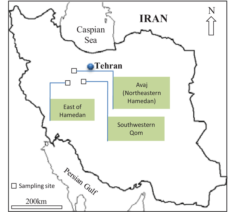
4. DATASET
One of the key steps in network designing is data collection. For this purpose, 10 sandstone blocks were selected from different locations in Central Iran and Sanandaj-Sirjan zones (Fig. 1). These sandstones belong to the upper red formation in southwest Qom and northeast Hamedan, and Jurassic sandstones in the east of Hamedan. Then, the collected blocks were cored in the laboratory to prepare core samples with NX size (54.1 mm diameter) based on the ISRM [1]. To develop the ANN model, different engineering properties (physical or mechanical) of 60 sandstone samples such as UCS, Schmidt hardness, P-wave velocity, porosity, and dry density were determined according to the ISRM [1]. The study by Momeni et al. [9] shows that there should be a good correlation between the input parameters and the model output. Hence, in this study, apart from UCS, other properties (which are related to UCS) were set as model inputs based on an extensive literature review (Tables 1 and 2). The results of the laboratory tests of selected samples are listed in Table 3. As presented in this table, the porosity values of studied sandstones range from 2.19 to 14.51%. The P-wave velocity of samples varies between 1.09 and 5.38 km/sec. The results for dry density show that γd range from 2.04 to 2.94 gr/cm3. Also, the Schmidt hardness number for selected sandstones varies between 23 and 46. The results of this work indicate that the UCS values range from 29.94 to 143 MPa.
| Sample No. |
Porosity (%) |
P-wave Velocity (km/sec) |
Dry Density (gr/cm3) |
Schmidt Hardness |
UCS (MPa) |
|---|---|---|---|---|---|
| 1 | 12.32 | 2.01 | 2.14 | 32 | 35 |
| 2 | 13.94 | 1.78 | 2.12 | 29 | 31 |
| 3 | 6.94 | 2.31 | 2.54 | 44 | 59.22 |
| 4 | 6.91 | 4.22 | 2.76 | 45 | 96.11 |
| 5 | 2.54 | 5.32 | 2.93 | 45 | 132.02 |
| 6 | 3.57 | 4.53 | 2.82 | 42 | 115 |
| 7 | 3.5 | 4.34 | 2.81 | 30 | 111.13 |
| 8 | 11.9 | 1.21 | 2.12 | 30 | 33 |
| 9 | 14.5 | 1.42 | 2.21 | 43 | 36 |
| 10 | 7.3 | 2.78 | 2.63 | 43 | 66.7 |
| 11 | 3.23 | 4.87 | 2.83 | 33 | 119.4 |
| 12 | 5.60 | 2.62 | 2.49 | 34 | 67.52 |
| 13 | 4.01 | 4.87 | 2.86 | 39 | 116.68 |
| 14 | 7.89 | 2.34 | 2.46 | 27 | 46.32 |
| 15 | 14.51 | 1.09 | 2.15 | 38 | 29.94 |
| 16 | 2.71 | 5.21 | 2.89 | 30 | 127.12 |
| 17 | 7.90 | 2.21 | 2.46 | 46 | 42.21 |
| 18 | 2.19 | 5.38 | 2.94 | 28 | 143 |
| 19 | 5.81 | 3.73 | 2.66 | 38 | 86.93 |
| 20 | 13.2 | 1.32 | 2.17 | 44 | 34.5 |
| 21 | 6.26 | 3.81 | 2.66 | 26 | 92.61 |
| 22 | 12.57 | 1.22 | 2.04 | 39 | 30.38 |
| 23 | 7.13 | 3.37 | 2.67 | 39 | 84.58 |
| 24 | 9.18 | 2.51 | 2.6 | 44 | 68.63 |
| 25 | 12.24 | 1.91 | 2.54 | 35 | 44.82 |
| 26 | 5.81 | 4.30 | 2.68 | 26 | 89.42 |
| 27 | 7.48 | 3.19 | 2.65 | 44 | 82.71 |
| 28 | 4.71 | 4.72 | 2.81 | 43 | 106.68 |
| 29 | 10.11 | 2.29 | 2.6 | 40 | 60.83 |
| 30 | 6.73 | 4.04 | 2.72 | 32 | 90.8 |
| 31 | 5.61 | 4.37 | 2.77 | 29 | 99.48 |
| 32 | 4.64 | 4.65 | 2.87 | 44 | 112.13 |
| 33 | 7.48 | 2.83 | 2.57 | 45 | 69.97 |
| 34 | 3.28 | 4.76 | 2.84 | 42 | 114.22 |
| 35 | 4.58 | 4.96 | 2.14 | 30 | 110.75 |
| 36 | 6.27 | 4.45 | 2.76 | 40 | 95.06 |
| 37 | 2.65 | 4.23 | 2.85 | 23 | 130.21 |
| 38 | 6.29 | 4.41 | 2.73 | 32 | 94.78 |
| 39 | 7.62 | 3.25 | 2.67 | 32 | 82.57 |
| 40 | 8.26 | 2.66 | 2.6 | 29 | 78.2 |
| 41 | 6.33 | 3.15 | 2.69 | 28 | 82.77 |
| 42 | 8.9 | 2.48 | 2.58 | 31 | 75.23 |
| 43 | 13.23 | 1.74 | 2.51 | 32 | 38.32 |
| 44 | 11.25 | 2.08 | 2.57 | 33 | 51.32 |
| 45 | 7.53 | 2.98 | 2.7 | 26 | 89.47 |
| 46 | 8.42 | 2.34 | 2.61 | 40 | 64.21 |
| 47 | 10.11 | 1.94 | 2.48 | 42 | 44.8 |
| 48 | 9.01 | 2.07 | 2.69 | 35 | 49.28 |
| 49 | 7.71 | 2.42 | 2.55 | 34 | 53.76 |
| 50 | 10.61 | 1.72 | 2.54 | 43 | 40.32 |
| 51 | 9.11 | 1.8 | 2.56 | 42 | 42.56 |
| 52 | 7.81 | 2.56 | 2.74 | 40 | 56 |
| 53 | 7.41 | 2.82 | 2.76 | 33 | 60.48 |
| 54 | 9.21 | 2.35 | 2.67 | 44 | 44.64 |
| 55 | 7.71 | 2.99 | 2.76 | 43 | 63.36 |
| 56 | 6.96 | 3.18 | 2.78 | 45 | 65.2 |
| 57 | 9.72 | 2.04 | 2.69 | 37 | 47.36 |
| 58 | 9.18 | 2.15 | 2.69 | 41 | 49.12 |
| 59 | 7.15 | 2.28 | 2.62 | 34 | 51.36 |
| 60 | 6.73 | 2.36 | 2.6 | 35 | 53.6 |
5. MODELLING PROCEDURE
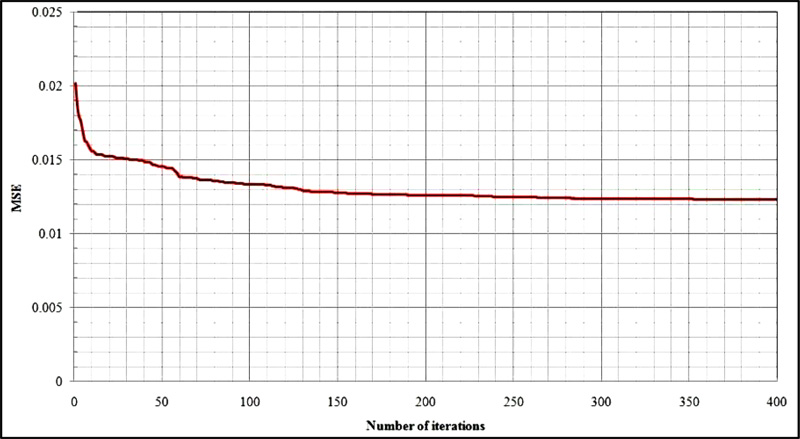
The modelling procedure of the PSO-based ANN predictive model starts with data normalization and sensitivity analysis. In fact, one may perform different sensitivity analyses in order to obtain the proper PSO parameters. In this study, the number of iterations was set to be the termination criterion for the hybrid model. For this reason, using a sensitivity analysis, firstly, the number of iterations was set to 400 and then the prediction performance of the model was evaluated using mean square error. Fig. (2) shows the effect of the number of iterations on the model response. As shown in this model, after nearly 50 iterations there is no significant change on the MSE; therefore, the maximum number of iterations was set to be 50. The values of C1 and C2 were set to be 2 according to the literature. The study by Tonnizam Mohamad et al. [39] recommends that the swarm size does not have a remarkable effect on the model performance; hence the number of particles in this study was set to 200.
After proper determination of the PSO parameters, the structure of the main ANN model (i.e. number of hidden nodes) has to be configured. In this regard, two methods are recommended in the literature. Some studies recommend using a trial and error procedure for determining the proper number of hidden nodes. On the other hand, some studies suggest the implementation of a number of equations for hidden node determination. These equations are related to the number of inputs and output(s). In this study, based on the authors' experience, the trial-and-error method was implemented. In other words, the models were trained and tested with three, four and five hidden nodes, respectively and the prediction performances were evaluated based on R2 as well as Root Mean Square Error (RMSE).
It is worth mentioning that each model was trained and tested five times. Since increasing the number of hidden nodes can lead to model complexity, in this study, a maximum of five hidden nodes in a hidden layer were used for training the model. It should also be mentioned that 80 percent of the data was used for training the model and the remaining 20% of the data was set for testing the model performance.
Table 4 shows the results of the implemented trial and error procedure for determining the best network architecture. It is worth mentioning that the prediction performance of the testing data was considered as the main criterion for the selection of the best model. Table 4 shows that the prediction performances of all models are close to each other meaning that the likelihood of accidental good results is negligible. When results for different hidden nodes are close to each other, to have a less complex model, one may select the model with the lowest hidden node more especially when the size of the dataset is not large. Hence, in this study, the 5th PSO-based ANN predictive model of UCS with three hidden nodes is selected as the best model.
6. RESULTS AND DISCUSSION
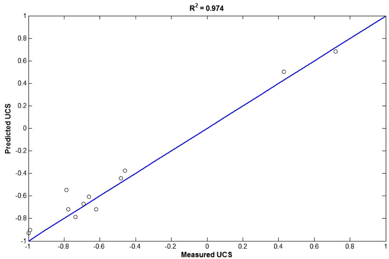
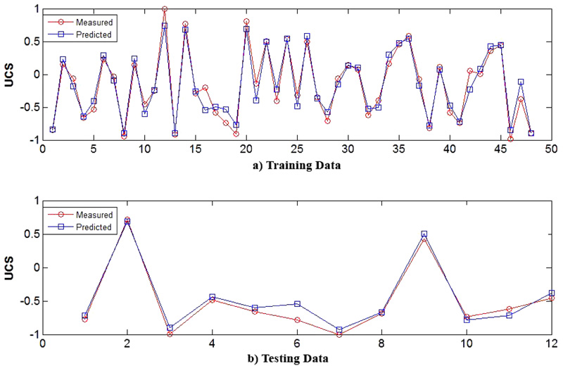
Figs. (3-5) indicate the reliability of the constructed PSO-based ANN model. Fig. (3) plots the predicted UCS values (in the training step) versus the measured UCS values in the laboratory. As shown in this figure, the coefficient of determination of the model for the training step is 0.941 which suggests the reliability of the model. As demonstrated in Fig. (4), the estimated UCS using the PSO-based ANN model for testing data is close to the measured UCS (R2=0.974), which indicates the relatively high reliability of the constructed network. As mentioned before, the coefficient of determination of more than 0.9 indicates that the predicted and measured values are in good agreement. Hence, based on the aforementioned results the predictive model of UCS is a feasible tool in predicting the UCS. It should be highlighted that implementations of such low- cost predictive models are simple and quick compared to direct or indirect methods of UCS estimation. However, the model should not be generalized when the estimated range of geomechanical properties are beyond the range of the presented data in Table 3. The proper prediction performance of the PSO-based ANN technique to estimate the UCS during training and testing steps is also shown in Fig. (5) for both training and testing data. As displayed in this figure, the predicted UCS values using the constructed network are close to the measured values, which indicate the reliability of the proposed PSO-based ANN model.
| Number of Nodes | 3 | 4 | 5 | |||||||||
|---|---|---|---|---|---|---|---|---|---|---|---|---|
| Model Number | R2 | RMSE | R2 | RMSE | R2 | RMSE | ||||||
| Test | Train | Test | Train | Test | Train | Test | Train | Test | Train | Test | Train | |
| I | 0.964 | 0.948 | 0.467 | 0.109 | 0.96 | 0.942 | 0.38 | 0.387 | 0.98 | 0.944 | 0.469 | 0.114 |
| II | 0.90 | 0.946 | 0.469 | 0.122 | 0.98 | 0.94 | 0.007 | 0.130 | 0.91 | 0.96 | 0.146 | 0.110 |
| III | 0.980 | 0.942 | 0.140 | 0.114 | 0.964 | 0.944 | 0.08 | 0.130 | 0.97 | 0.946 | 0.100 | 0.122 |
| IV | 0.946 | 0.948 | 0.109 | 0.126 | 0.946 | 0.952 | 0.126 | 0.114 | 0.98 | 0.942 | 0.086 | 0.119 |
| V | 0.974 | 0.941 | 0.089 | 0. 126 | 0.904 | 0.940 | 0.14 | 0.13 | 0.976 | 0.947 | 0.097 | 0.119 |


In this study, for comparison purposes, Multiple Linear Regression (MLR) method is also implemented for the prediction of UCS. Same dataset and input parameters were used in the MLR-based predictive model. To produce a multivariate equation, the statistical software package SPSS23 was used. Lastly, the best obtained multivariate regression equation is suggested for UCS estimation (Eq. 3).
 |
(3) |
Fig. (6) shows the correlations between the estimated values of the UCS using MLR method (Eq. 3) and the observed values in the laboratory for both training and testing data. On the basis of the results, the R2 between the predicted and observed UCS for training and testing steps are 0.940 and 0.966, respectively. Hence, it can be concluded that the MLR is also capable of forecasting UCS with acceptable precision. However, the use of the PSO-based ANN predictive model of UCS is more preferable.
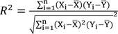
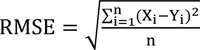
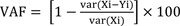
As mentioned earlier, the prediction performances of the developed models were assessed using different standard statistical indices including the R2, and Root Mean Square Error (RMSE). At the final stage, Variance Accounts For (VAF) was also utilized for comparing both predictive models. The aforementioned performance indices were calculated using the following equations:
 |
(4) |
 |
(5) |
 |
(6) |
| Proposed Model | Model Reliability | - | - | - |
|---|---|---|---|---|
| - | R2 | R2 | RMSE | RMSE |
| - | (training data) | (testing data) | (training data) | (testing data) |
| MLR-based Predictive model of UCS | 0.931 | 0.966 | 0.106 | 0.094 |
| PSO-based Predictive model of UCS | 0.941 | 0.974 | 0.126 | 0.089 |
Where Xi and Yi are the observed and predicted data, respectively;
 and
and
 are mean of the measured and predicted data, and n is the number of data points. As previously mentioned, in theory, an estimation model is excellent when R2 is 1, RMSE is equal to 0 and VAF is 100. The values of the aforementioned statistical indices are tabulated in Table 5. The performance indices values shown in this table suggest that the PSO-based ANN model outperforms the MLR-based predictive model of UCS; therefore, this study recommends the implementation of the PSO-based predictive model as a feasible tool for estimation of UCS. However, further research is suggested for model generalization.
CONCLUSION
In this study, using 60 datasets, two predictive models of UCS were proposed. Porosity, P-wave velocity, dry density and Schmidt hardness number were set to be model inputs. Based on the results, it was concluded that the PSO-based ANN model with three hidden nodes performs good enough in assessing the UCS of sandstone. A comparison between the prediction performance of the intelligent-based predictive model and MLR-based predictive model showed that the PSO-based ANN model outperforms the MLR-based predictive model. However, it should be highlighted that the proposed predictive models work well enough when the future data are in the range of the data presented in Table 3. Further research with the larger dataset is recommended for overcoming the aforementioned limitation.
CONSENT FOR PUBLICATION
Not applicable.
AVAILABILITY OF DATA AND MATERIALS
Not applicable.
FUNDING
None.
CONFLICT OF INTEREST
The authors declare no conflict of interest, financial or otherwise.
ACKNOWLEDGEMENTS
Declared none.