All published articles of this journal are available on ScienceDirect.

ARMA Models to Measure the Scale of Fluctuation from CPT Data
Abstract
Objective:
Spatial variability is one of the largest sources of uncertainty in geotechnical applications. This variability is primarily characterized by the scale of fluctuation, a parameter that describes the distance over which the parameters of a material are similar. Spatial variability is generally described with traditional methods of time series analysis. In statistics, the Auto-Regressive Moving Average (ARMA) model is commonly used to describe the relationship between two points in time. Instead of assuming an autocorrelation model, the ARMA model calculates the necessary auto-regressive components (AR), as well as a decaying Mean Structure (MA). The advantage of this method is that it is calculated for each specific field study, so that the data is not forced to fit into a fixed autocorrelation model (e.g. Markovian, Gaussian, etc).
Methods:
In this study, the ARMA model is introduced as a means of measuring scale of fluctuation, and two case studies and a simulation are used to compare the scale of fluctuation values from the ARMA model to the other estimates.
Results:
In the first case study, the ARMA model estimated a value of 0.26 m while the other methods ranged from 0.22-0.29 m. In the second case study, the ARMA model estimated a value of 0.40 m while the other methods ranged from 0.40-0.54 m. In the simulated example, where the true value was 5.0 m, the ARMA model estimated a value of 4.73 m while the other methods ranged from 3.24-3.51 m.
Conclusion:
This paper concludes that ARMA is a promising new method for estimating the scale of fluctuation but requires a considerable amount of research before it can become established in the geotechnical sphere.
1. INTRODUCTION
Spatial variability is one of the largest sources of uncertainty in geotechnical applications. In recent decades, the necessity of considering spatial variability in geotechnical applications has been demonstrated in various studies [1-19]. This variability is primarily characterized by the scale of fluctuation which describes the distance over which the parameters of a soil or rock are similar or correlated; soil properties sampled from adjacent locations in the soil profile tend to have similar values and as the sampling distance increases, the correlation decreases. It is required to characterize as well as simulate a spatially variable field. It should be noted that a different scale of fluctuation is defined for each material, so the CPT data considered here is material-specific. Due to the importance of the scale of fluctuation, various methods have been developed to characterize this parameter from soil data, particularly Cone Penetration Test (CPT) measurements, the most commonly used method of obtaining near continuous field data. The scale of fluctuation can be estimated from CPT data using methods such as the method of moments [20-23], maximum likelihood estimation [24-26], and Bayesian analysis [27, 28].
Spatial variability is generally described by traditional methods of time series analysis in statistics, meaning that it constitutes a trend component and a zero-mean spatial variability component (Equation 1). The reason for this is that as with measurements in time, soil property measurements that are closer together in space are more similar in value, as shown below:
 |
(1) |
where Xi is the value of the soil property at location Si, Si is the vertical distance from the ground surface, for example, and k is the total number of measurements. ϵ(Si) is the spatial variability component. The scale of fluctuation describes the distance over which the spatial variability components ϵ(Si) are correlated amongst themselves.
The commonly used methods of measuring the scale of fluctuation in the geotechnical field assume an autocorrelation model. A method of moments can then be used to estimate the scale of fluctuation value, by minimizing the error between the theoretical autocorrelation model and the experimental one [29]. An autocorrelation model describes the relationship between the distance separating two points and the correlation between them. Some typical autocorrelation models are shown in Table 1, where ρ(τ) is the correlation coefficient between two points separated by lag τ, θ and is the scale of fluctuation.
| Autocorrelation Model | Relationship |
|---|---|
| Markovian |
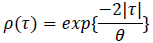
|
| Gaussian |
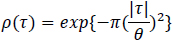
|
| Spherical |
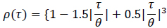
|
1.1. Need for Research
In the current typical methods to measure the scale of fluctuation, the autocorrelation model selected for a given set of CPT measurements is generally just assumed to be the one that describes the true structure of the data. Since no model can fit the data exactly, this makes the selection of an autocorrelation model difficult.
In statistics, the Auto-Regressive Moving Average (ARMA) model is commonly used to describe the relationship between two points in time. Instead of assuming an autocorrelation model, the ARMA model calculates the necessary auto-regressive components (AR), as well as a decaying mean structure or Moving Average (MA). The advantage of this method is that it is calculated for each specific field study, so that the data is not forced to fit into a fixed autocorrelation model. Additionally, a very simple and fast algorithm is needed to calculate the necessary AR, and MA coefficients.
In this study, the ARMA model is introduced as a means of measuring the scale of fluctuation. Two case studies and a simulation are used to compare the scale of fluctuation values from the ARMA model to the method of moments estimates. There are no previous studies that used this method to measure the scale of fluctuation.
2. MATERIALS AND METHODS
2.1. ARMA
2.1.1. Stationary Time Series
As with the methods of moments, in order to measure the scale of fluctuation from CPT data, the data must first be stationary. A stationary time series has properties that do not depend on the time at which the series was observed. In the CPT realm, a stationary CPT is one whose properties do not depend on the depth.
Weakly stationarity is defined by a constant mean, variance, and covariance structure. This is necessary in order for the autocorrelation function to have meaning. While the constant variance and covariance must be assumed, the constant mean is the famous de-trending problem. This is analogous to removing the trend of measurement and only looking at the spatial variability component ϵ(Si) in Equation 1). The readers are referred to the multitudes of literature on the subject, some of which are included here [30-32]. The data used in the remainder of the paper is assumed to satisfy weakly stationarity.
2.1.2. The ARMA Model
The Auto-regressive (AR) component of the ARMA model allows for current measurements in time to depend on a certain lag of past measurements. For example an AR(1) model indicates that the current measurement depends on the last. An AR(2) model indicates that the current measurement depends on the last and the one previous to that. This can be similarly applied to CPT measurements, such that for an AR(2) model, a measurement at a given location depends on the measurements at the two previous locations adjacent to it. An AR(p) model is expressed as shown in Equation 2 below, where αi are the coefficients associated with each past measurement, and wi are the random error components which are typically assumed to independently and identically distribute white noise with some fixed variance σ22. Xi is the value of the soil property at location Si, Xi-1 is the value at location Si-1, and δ is the intercept.
 |
(2) |
The Moving Average (MA) component indicates that the regression error is a linear combination of the error terms at the previous locations. Similarly to the AR, an MA(2) model indicates that the current error depends on the error at the previous two locations. An MA(q) model is expressed as shown in Equation 3 below, where θi are the coefficients associated with each past measurement error, wi-1 is the error associated with measurement Xi-1, and is the intercept.
 |
(3) |
Therefore, for stationary data, an ARMA(p,q) model can be expressed as shown in Equation 4 below, where p is the order of the AR component, and q is the order of the MA component:
 |
(4) |
In the equation above, Xi are the stationary measurements at each location, αi are the coefficients of the AR components, θi are the coefficients of the MA components, and wi are the errors associated with the MA model.
Once the coefficients αi and θi are determined for the necessary number of p and q, then the autocorrelation function for the specific case is defined, and the scale of fluctuation can be calculated as simply the area under the correlation function.
It turns out that these coefficients and orders can be determined automatically and quickly with a simple algorithm.
2.1.3. Determining the ARMA coefficients
There are two ways to determine the ARMA coefficients. One is by visual inspection of the autocorrelation function and partial autocorrelation function plots. It is often evident from reviewing these plots what the values of p and q should be. An even simpler way is using the auto.arima algorithm from the forecast package in R [33, 34]. This code is open-source and available for implementation in other software.
The auto.arima function takes as an input the CPT data in the format of measurement locations and measurements at each location. It outputs the necessary values for p and q and their respective coefficients.
Once the numbers of terms are known (p and q), the coefficients themselves are determined as would be done for any regression equation. The auto.arima algorithm determines these coefficients as well.
Once these coefficients are determined, the correlation structure of the data is explained.
2.1.4. Determining the Scale of Fluctuation
Once the coefficients are determined, the autocorrelation function ρ(τ) can be defined and the corresponding scale of fluctuation, θ, is the area under this function, as shown in Equation 5 [29]:
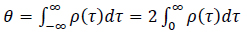 |
(5) |
An important note is warranted here – the factor of 2 in the equation above is often omitted hence resulting in two definitions of the scale of fluctuation. What is alternately referred to as scale of fluctuation or correlation length has been defined as both θ and θ/2 in geotechnical literature, resulting in confusion. In this study, the scale of fluctuation refers to θ as defined above.
This integral can be easily obtained with the quadrature of the autocorrelation function.
3. VERIFICATION
Three examples are considered for verification of the ARMA method. The first two use CPT measurements from two studies, the scale of fluctuations of which were measured using a method of moments and an assumed autocorrelation model. These are used to verify that ARMA gives similar results to classic methods. The third example is a simulated example where the scale of fluctuation is known, and ARMA as well as methods of moments are used to see how close they can get to the true measurement.
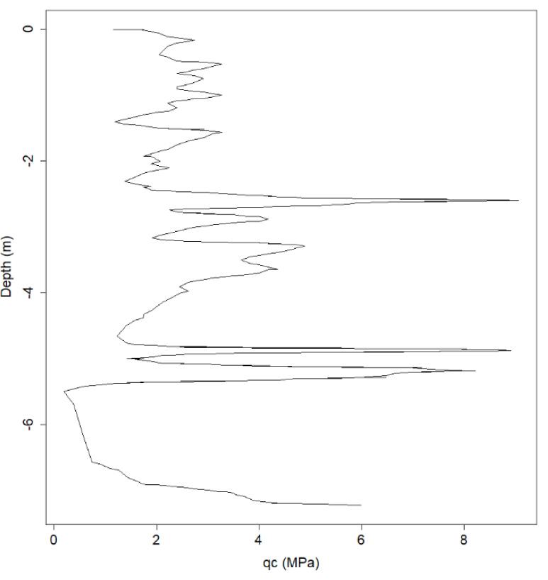
3.1. Example 1: Świebodzice
This example uses a CPT measurement from Świebodzice [35], the scale of fluctuation of which was measured by Pieczyńska-Kozłowska (2015) [36]. The Świebodzice CPT for qc used in the study is shown in (Fig. 1).
Pieczyńska-Kozłowska (2015) [36] used various autocorrelation models and de-trending methods and compared the resulting scale of fluctuations, measured using methods of moments. For comparison purposes, only the linearly de-trended measurements are used below. These results form Pieczyńska-Kozłowska (2015) [36] are summarized in Table 2.
| Markov Autocorrelation | Gaussian Autocorrelation | |
|---|---|---|
| Vanmarcke Method | 0.28 m | 0.22 m |
| Rice Method | 0.23 m | 0.29 m |
The auto.arima function from the forecast package determined that an ARMA(4,4) (for more details please see section 2.3) model best described the correlation structure. That is, a model with 4 AR terms and 4 MA terms. The coefficients of this model are as shown in Table 3. Using these coefficients and quadrature of the resulting autocorrelation function as explained in section 2.2, the estimated scale of fluctuation was found to be 0.26 m, which is in close agreement with the values found by Pieczyńska-Kozłowska (2015) [36].
| AR Coefficients, αi | MA Coefficients, θi |
|---|---|
| 0.83 | 0.17 |
| 0.25 | 0.29 |
| 0.53 | -0.34 |
| -0.63 | 0.34 |
3.2. Example 2: Taranto Clay
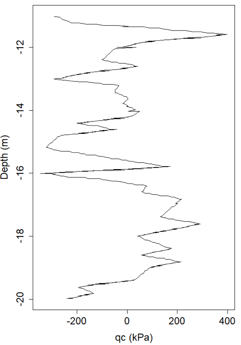
The second example uses a CPT measurement from Taranto, Italy [37]. The G1 borehole of the lower clay data is used for comparison purposes, as de-trended (see section 2.1) by Cafaro and Cherubini (2002) [37]. This de-trended data is shown in (Fig. 2).
Cafaro and Cherubini (2002) [37] used the variance function method to measure the scale of fluctuation and obtained a value of 0.536 m for the specific borehole, with an average measurement of 0.40 m over the five boreholes. The auto.arima function determined an ARMA (2,1) model to be the best fit for borehole G1, the coefficients of which are shown in Table 4. The estimated scale of fluctuation was found to be 0.40 m. This is in close agreement with the estimated measurement for the given borehole as well as the average over the five boreholes.
| AR Coefficients, αi | MA Coefficients, θi |
|---|---|
| 1.98 | -0.90 |
| -0.98 | - |
3.3. Example 3: Simulated Data
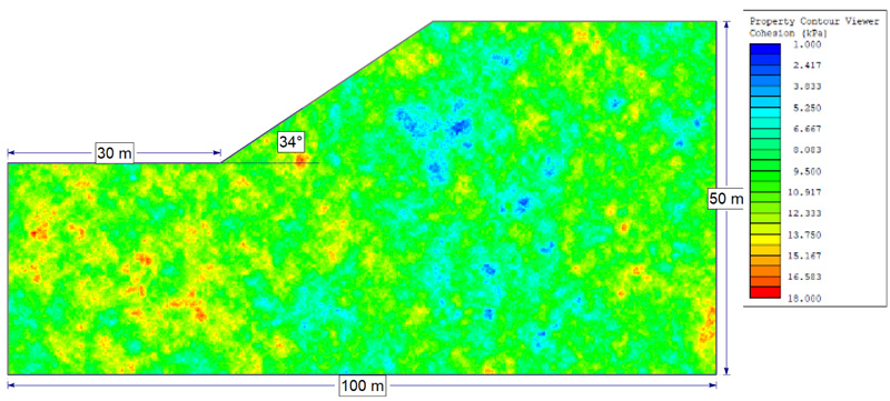
Finally, the third example uses data that was simulated to have a scale of fluctuation of 5 m. This was done using the spatial variability field option in the Slide2 software [38], which uses Markovian and Gaussian autocorrelation functions together with a method known as Local Average Subdivision (LAS) to generate the field. The simulated field is a spatially variable cohesion parameter with a mean of 10 kPa, a standard deviation of 2 kPa, and a normal distribution. The spatial field with a mesh size of 0.2 m in a typical slope with a unit weight of 19 kN/m3 and a friction angle of 23 degrees is shown in (Fig. 3).
Five relatively equi-spaced vertical samples were taken from the field, at x=1.1 m, x=20 m, x=50.1 m, x=75.1 m, and x=98.3 m. The scale of fluctuation was measured using both ARMA and an autocorrelation fitting method along with Markovian and Gaussian autocorrelation models. Since this data is simulated, de-trending was not necessary. The results are summarized in Table 5.
This simulated example has attempted to replicate what might happen in the field, where only a handful of boreholes are taken and must be used in order to characterize the field. It is seen that although all methods in Table 5 tend to deviate from the true value at specific locations, when averaged, the ARMA model gives a value that is much closer to the 5 m measurement. This is due to the fact that ARMA defines an autocorrelation model for each of the five locations exactly, instead of assuming the Markovian or Gaussian autocorrelation model.
| Measurement Location | Autocorrelation Fitting with Markovian Model | Autocorrelation Fitting with Gaussian Model | ARMA |
|---|---|---|---|
| 1.1 | 3.32 m | 3.36 m | 5.58 m |
| 20 | 1.77 m | 1.36 m | 1.65 m |
| 50.1 | 5.32 m | 6.41 m | 6.60 m |
| 75.1 | 3.51 m | 3.92 m | 6.27 m |
| 98.3 | 2.26 m | 2.47 m | 3.58 m |
| Average | 3.24 m | 3.51 m | 4.73 m |
These three average scales of fluctuations were input into a spatial variability analysis for the slope in (Fig. 3) using 500 Latin-Hypercube samples and Morgenstern-Price limit equilibrium method in order to get a rough idea of the expected difference in probability of failure when the scale of fluctuation is misrepresented.
It can be seen in the table that the scale of fluctuation parameter has a considerable effect on the probability of failure.
4. DISCUSSION
The ARMA model is a commonly used method in time series analysis which has not yet entered the geotechnical sphere. This may be due to the relatively recent introduction of statistics into geotechnical engineering, as well as the efforts required to determine the values of p and q. However, with statistics becoming a more integral part of a geotechnical analysis, and with open-source algorithms automating the determination of p and q, it is time that the ARMA model enters the geotechnical sphere.
This study serves as an introduction to ARMA in geotechnical engineering through an overview of the theory as well as real and simulated examples. While the results in this study have been positive, a considerable amount of research remains to be done.
CONCLUSION
In this study, the ARMA model is introduced as a means of measuring the scale of fluctuation. The advantage of this method is that it allows the autocorrelation model to be defined exactly, instead of forcing the data to fit into a pre-defined model such as Gaussian or Markovian. Additionally, an open-source algorithm is available for finding the coefficients of the model quickly and easily.
Two case studies and a simulation are used to compare the scale of fluctuation values from the ARMA model to the estimates of the method of moments. In the first case study, the ARMA model estimated a value of 0.26 m while the other methods ranged from 0.22-0.29 m. In the second case study, the ARMA model estimated a value of 0.40 m while the other methods ranged from 0.40-0.54 m. In the simulated example, where the true value was 5.0 m, the ARMA model estimated a value of 4.73 m while the other methods ranged from 3.24-3.51 m (Table 6). This has a considerable effect on the computed probability of failure.
CONSENT FOR PUBLICATION
Not applicable.
AVAILABILITY OF DATA AND MATERIALS
The CPT data supporting the findings of the article is available in the Pieczyńska-Kozłowska (2015) at https://content.sciendo.com/view/journals/sgem/37/4/article-p95.xml [36], and Cafaro and Cherubini (2002) at https://ascelibrary.org/doi/abs/10.1061/(ASCE)1090-0241(2002)128:7(558) [37].
FUNDING
None.
CONFLICT OF INTEREST
The authors declare no conflict of interest, financial or otherwise.
ACKNOWLEDGEMENTS
Declared none.