All published articles of this journal are available on ScienceDirect.

Evaluation of Seismic Demand for Substandard Reinforced Concrete Structures
Authors Info & Affiliations
Abstract
Background:
Reinforced Concrete (RC) buildings with no seismic design exhibit degrading behaviour under severe seismic loading due to non-ductile brittle failure modes. The seismic performance of such substandard structures can be predicted using existing capacity demand diagram methods through the idealization of the non-linear capacity curve of the degrading system, and its comparison with a reduced earthquake demand spectrum.
Objective:
Modern non-linear static methods for derivation of capacity curves incorporate idealization assumptions that are too simplistic and do not apply for sub-standard buildings. The conventional idealisation procedures cannot maintain the true strength degradation behaviour of such structures in the post-peak part, and thus may lead to significant errors in seismic performance prediction especially in the cases of brittle failure modes dominating the response.
Method:
In order to increase the accuracy of the prediction, an alternative idealisation procedure using equivalent elastic perfectly plastic systems is proposed herein that can be used in conjunction with any capacity demand diagram method.
Results:
Moreover, the performance of this improved equivalent linearization procedure in predicting the response of an RC frame is assessed herein.
Conclusion:
This improved idealization procedure has been proven to reduce the error in the seismic performance prediction as compared to seismic shaking table test results [1] and will be further investigated probabilistically herein.
1. INTRODUCTION
Although less accurate than Time History Analysis (THA), Capacity Demand Diagram Methods (CDDMs) have proven to be very efficient in predicting the inelastic deformation of buildings in many existing studies [1-6]. They are a valuable alternative to the tedious and computationally intensive THA for seismic performance estimation of large building populations clustered in classes. In brief, these methods transform the response of a nonlinear Multi Degree of Freedom (MDOF) system into an equivalent linear Single Degree of Freedom (SDOF) system and compare its response (capacity curve) to the earthquake demand expressed in the form of a response spectrum. CDDMs use predominantly equivalent linearization procedures based on flexural ductile response and only in some cases, account for the strength and stiffness degradation behavior in idealizing the capacity curve. In general,0 these methods use monotonic or cyclic induced displacements in both +ve and –ve directions of a 2D frame to compute pushover curves and derive the capacity of the structure. The Performance Point (PP) in terms of spectral displacement of the equivalent single degree of freedom system can then be found from the capacity curve with the use of a reduced elastic response spectrum. The reduction is applied either through an increase in the damping ratio resulting from damage of the structure or through the use of equations relating the behaviour factor (q) with the ductility (μ) for varying fundamental periods of vibration (T) of the equivalent SDOF system.
The limitations of CDDM’s in predicting the seismic demand are well described in [7] and are mainly related to the poor representation of the seismic hazard and the procedure for the estimation of the performance point. A wide use of these methods, especially in cases of risk assessment at country level, raises though the need to improve its accuracy and this is why both FEMA in [5] and ATC in [8] proposed modified or updated versions to account for strength and stiffness loss.
Accounting for the degrading behaviour of substandard systems mainly due to brittle failure modes, (which is the case for most existing structures designed prior to the enforcement of modern seismic codes) is a challenge when using these methods and their accuracy in seismic performance prediction will be examined herein. Guidelines by FEMA on the seismic rehabilitation of buildings (FEMA 273 [9], FEMA356 [10]) propose the Displacement Coefficient Method (DCM), in which a factor C2 accounts for the effect of strength and stiffness degradation and pinched hysteretic behaviour on maximum displacement response. Other CDDMs, such as the ones included in the ATC-40 [10] and FEMA440, also consider the degrading characteristics using different factors related to the equivalent hysteretic damping and ductility for specific hysteresis loop types. These factors depend on the quality of the structure (with respect to lateral resistance and hysteretic behaviour) and account for the variation of actual building hysteretic behaviour from the theoretical elastic-plastic (EP) behaviour. Based on hysteretic behaviour, structural systems in ATC-40 (1996) are divided into three categories A, B and C and a k value is assigned to each category. Category A represents Elastic Perfectly Plastic (EPP) behaviour, whereas category C represents a strongly pinched or poor hysteretic response. In the improved equivalent linearization procedure proposed in FEMA440 [4], equations are included for evaluating equivalent hysteretic damping in different ductility ranges in order to generate highly damped elastic response spectra. The coefficient values in these equations correspond to different post elastic stiffness ratios denoted as α-values of a particular hysteretic behaviour such as bilinear (BLN), stiffness degradation (STDG), and strength degradation (STRDG). One unique feature of this procedure in FEMA440 is that it accounts for the strength degradation hysteretic behaviour that could occur in the same cycle, in which yield occurs (in-cyclic degradation) and leads to a negative post yield stiffness. The use of negative post yield stiffness is crucial for the bi-linearization of the capacity curve of strength degradation systems, since it accounts for the loss of strength in the energy balance calculation.
For systems with significant strength loss though, part of the energy dissipation capacity is lost after the maximum load point, resulting in a significant reduction of hysteretic damping capacity and thus a single bilinear approximation of the capacity curve cannot account for this reduction. A procedure is proposed in this paper, which aims at improving even more the predictions of the FEMA440 [5] procedure through the detailed discretization of the capacity curve, to overcome this problem and account for the significant post peak strength loss of degrading systems; this proposed idealisation procedure can be applied in the context of any capacity demand diagram method, since it solely alters the prediction of the performance point and not the procedure to account for non-linearity. It is referred to as an idealisation procedure, since it tackles the problem of idealising a degrading capacity curve provided by push-over analysis. It is not by any means a capacity demand diagram method for the prediction of the structural response, but it can be used in conjunction with any capacity demand diagram method. The equivalent linearization procedure in FEMA440 is chosen herein to illustrate the proposed procedure. Nevertheless, the purpose of the paper is to illustrate the proposed idealisation procedure and not to compare different capacity demand diagram methods.
This paper initially describes the details and results of a full-scale shake table testing of a 2 storey 1 bay RC frame with no seismic design and deficient detailing. The test results (displacements) are then used to assess the performance of the existing FEMA440 capacity demand diagram method referred to as MADRS in predicting the seismic response (displacements). Further on, the proposed idealisation procedure is integrated in the MADRS method to assess the enhancement provided in performance prediction. The proposed idealisation procedure uses multiple Equivalent Elastic Perfectly Plastic (EEPP) systems rather than a single one, which is the standard practice in all CDDM’s, in order to include all the characteristics of the original degrading capacity curve of the transformed SDOF system.
In addition, in order to illustrate the effectiveness of the proposed idealisation procedure, a probabilistic study is conducted on typical deficient RC building classes found in developing countries. The performance predictions using the original idealisation procedure (MADRS) and the proposed one (MADRS and EEPP systems) are compared to results from THA.
2. CASE STRUCTURE FOR PERFORMANCE EVALUATION: ECO-LEADER BUILDING
2.1. Background
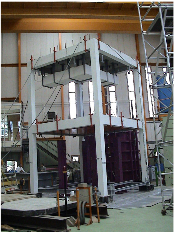
To assess the efficiency of CDDM’s in predicting seismic performance, the results of a 2 storey one bay full-scale RC frame (Fig. 1) tested on a shake table [11] are used in the first stage. Details of the test campaign and the results are included in [11].
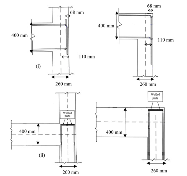
This RC frame was tested to various seismic acceleration time-history inputs with different PGA levels (0.05g, 0.1g, 0.2g, 0.3g, 0.4g). These time histories with a duration of 40 seconds were derived from Eurocode 8 [12] type-1 spectrum corresponding to the medium dense sand with a corner period Tc=0.6sec. The frame was designed according to old European codes, with mean concrete compressive strength of 20MPa, poor reinforcement detailing and no capacity design. Thus, the frame is regarded as a Gravity Loaded Design (GLD) frame having strong beams and weak columns with similar design, detailing and material characteristics of non-engineered reinforced concrete (NERC) structures [13] and thus violates the provisions of modern codes, such as Eurocode 2 [14] and Eurocode 8 [12], both as far its anchorage and shear capacity are concerned. The detailing of the frame members was supposed to simulate detailing provided by old codes enforced in the Mediterranean during the 1980s and 1990s. Main longitudinal column reinforcement bars were welded on short re-bar lengths for anchorage (Fig. 2b), following a common practice of that period. The beam reinforcement anchorage (Fig. 2a) was provided in accordance to [15] which is still regarded as deficient compared to the provisions of modern seismic codes. The spacing of the links was 200mm in the columns and 300mm in the beams throughout their length in accordance to old construction practice, which is considerably inadequate even as maximum spacing by modern seismic design codes and may lead to both shear and buckling failures. In addition, and most importantly, no capacity design was applied to the frame as modern codes prescribe and, thus, beam sections have larger cross-sections than columns. Fig. (2) shows the design and as build anchorage details.
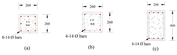
The frame was tested at the CEA facilities in Saclay, France, under the European Union (EU) project Eco-leader which enabled access to users (including the University of Sheffield) to these specialized shake table facilities [11]. The main aim of the project was to evaluate retrofitting strategies for the damaged RC structures. Initially the test was conducted on the bare frame at the above mentioned increasing PGA levels. The testing was repeated after it was retrofitted using carbon fibre reinforced polymers (CFRP’s) [11]. Cross-section details for columns and beams are shown in Figs. (3a, c). Material details are given in Table 1, and it should be noted that elongation (A %) refers to the elongation at mid-point of the bar where necking occurs and not at the ultimate steel strain which is used for analysis purposes. The corresponding strength capacities (flexural and shear) of the columns were obtained using section analysis, and corresponding factored axial loads are given in Table 2. To obtain the shear capacity the moment distribution in the columns was assumed triangular with point of contra-flexure in the midpoint of the column.
| Steel | |||
|---|---|---|---|
| Bar Diameter (mm) |
Yield Strength (MPa) |
Ultimate Strength (MPa) |
Elongation A% |
| 8 | 582 | 644 | 25 |
| 14 | 551 | 656 | 23.6 |
| Concrete | |||
| Mean compressive strength (MPa) |
Tensile strength (MPa) |
Elastic modulus (MPa) |
|
| 1st Floor: | 22.1 | 2.1 | 25590 |
| 2nd Floor: | 19.6 | 2.07 | 23500 |
| Strength Capacities | ||||||
|---|---|---|---|---|---|---|
| Floor Number | Md (kNm) | My (kNm) | Mult (kNm) | Fd (kN) | Fy (kN) | Fult (kN) |
| Floor 1 | 41 | 60 | 80 | 100 | 145.5 | 194 |
| Floor 2 | 25 | 37 | 46 | 61 | 90 | 111.5 |
2.2. Observed Damaged Patterns
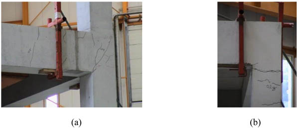
Based on the recorded damage observations [11], it can be concluded that most cracks were located close to the column-joints interfaces and in the joint. Moreover, very few cracks were also observed in the beams. No visible damage was observed after the first two seismic tests (0.05g and 0.1g) although an increase in period was recorded implying stiffness reduction due to cracking. During the 0.2g test, visible diagonal cracking appeared on the 1stfloor joints (Fig. 4a) along with horizontal cracking at the base of the second floor column and at the column interface below the 2ndfloor joint as shown in Fig. (4b).
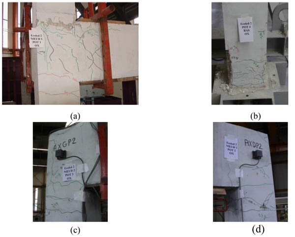
At 0.3g some new horizontal cracks were added at the top interface of the 1st floor joint, at the mid span of 1st floor columns and at the base of a single column as shown in Figs. (5a, b). Finally, during the last test (at 0.4g), cracking was visible on a column between the base and the first level. In addition, spalling of concrete occurred at the base of the column, where horizontal cracks were formed during the previous test (0.3g), as shown in Fig. (5b). The horizontal cracks at the column-joint interface became wider as shown in Figs. (5c, d). The top node displacements of the Eco-leader building at different PGA levels are given in Table 3.
| PGA (g) | 0.05 | 0.1 | 0.2 | 0.3 | 0.4 |
| Top Node Displacement (m) | 0.0170 | 0.0295 | 0.0820 | 0.1715 | 0.2212 |
A capacity-demand analysis of the Eco-leader building [3], showed that at the 0.2g test, the shear force demand on the first and second floor columns exceeded the column yield capacities (Fy) given in Table 2 leading to the conclusion that yielding of the column steel reinforcement was reached. In this analysis, maximum shear force as calculated using the flexural capacity of columns Table 2 is compared with the shear demand on columns expressed by the shear force time-histories at each floor. The same analysis showed that at the 0.4g test the column ultimate capacity (Fu) at the 1st floor columns was not reached and the estimated demand remained close to Fy. This observation raised the suspicion of possible existence of a failure mechanism other than flexure which created softening of the frame. In view of the above observation, and to further investigate this post yield softening response of the frame, the recordings from strain gauges at different locations were examined. The locations of the strain gauges are given in Fig. (6a). Since visible damage occurred at 0.2g (Fig. 4) and the shear demand has exceeded column yield capacities at both levels, the strain histories were examined for the remaining 2 excitation levels.
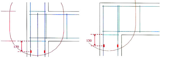
2.3. Description of Strain History Results
The strain gauge code numbers and magnitude located on columns (Col), along with the column numbering and are shown in Fig. (6a). In addition, their positions along the height of the columns are shown in Fig. (6b) for strain gauges located on 1st and 2nd floor columns respectively. At the 0.2g test, only the strain history from the 1st floor column strain gauge (JPOT-3) provided reliable recordings. The strain from JPOT-3 showed that the bars were still in the elastic range at 0.2g and the same was noticed at the higher PGA levels of 0.3g and 0.4g. However, the strain gauge JPOT-2 placed in the opposite first floor column (look at small schematic on Fig. (6a) has exceeded the yield strain limit at 0.3g and 0.4g by a small amount, which indicates no significant strain hardening. The peaks in the strain histories of JPOT-2 at 0.3g and 0.4g occur at the same time as the peaks in the displacement histories for the first floor, which is expected when the response of the floor is governed by flexural behaviour.
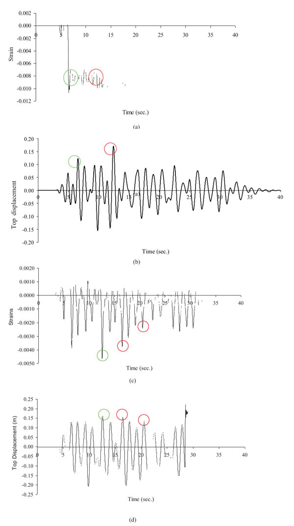
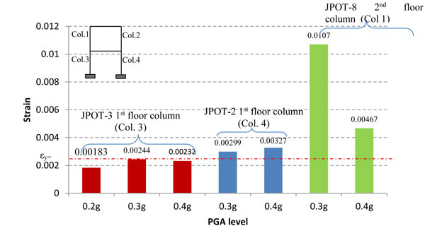
For the second floor, strain history results were not available for 0.2g, so only the 0.3g and 0.4g strain history results are shown in Fig. (7) and both values exceed the yield strain (εy=0.002). The strain gauge is located at a longitudinal main steel bar located in column 1 close to the interface with the joint and more information regarding the location of this strain gauge can be found in [11]. At 0.3g, the strain gauge JPOT-8, reaches a large strain at 6.6 sec and again at 12.4 sec. These strain peaks at both times are almost the same but the displacement at 6.6 sec is lower than the one at 12.4 sec, which indicates that accumulation of displacement at 12.4 sec may be a result of other softening mechanisms. Although the displacement of the frame at 12.4sec is higher, no additional strains were observed at the strain history. The strain history of the same strain gauge at 0.4g Fig. (7c) shows the yielding of reinforcement is also consistent with the peak displacement (Fig. 7d). However, the residual strain levels at subsequent yielding are considerably lower than expected from approximately equal displacement levels as the first yielding, which may indicate loss of bond.
To determine whether softening behaviour took place in the columns, it is necessary to undertake global time-history analysis with the incorporation of sophisticated models capable to account for bar slip deformations that may have resulted from loss of bar anchorage. The calibration of such models and the results of the analysis are shown in the next section. An extensive presentation of the models used for the analysis can be found in [1], [3], and [6].
3. MODELLING OF ECO-LEADER BUILDING
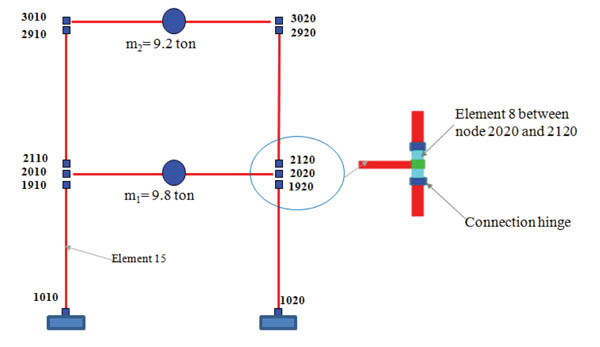
The structural members of the tested frame were modelled in the numerical analysis software Drain 3dx [17] as a 2D frame, since it was a symmetrical frame. The total mass of the frame was computed by adding the mass of the frame members to the imposed floor mass from metal plates. The metal plates were placed to simulate the imposed load on floors of real structures. For modelling purposes, the frame was analysed in two dimensions and the total floor mass was lumped at the mid-point of each floor beam, as shown in Fig. (8). The four-digit numbers at the joint and close to the column-joint interface are node numbers of the numerical model and represent the boundaries (beginning and end) of the connection hinge and the shear element used to model slip and shear deformations. The columns and beams were modelled using line fiber elements (element 15) and the sections were divided into a number of concrete and steel bar fibres. The connection hinge was used to account for the slip deformation and element 8 was used to include the effect of joint shear deformation. Details of the frame and element modelling can be found in [1], [3] as well as the calibration of the models to the test results described in the previous section. The Drain 3dx model for the Eco-leader building is shown in Fig. (8). The low strength concrete (LSC) stress-strain model (a modified Mander model) [18] was used to model the non-linear concrete behaviour.
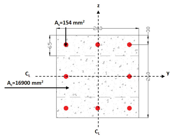
An example of the section discretization process is given in Fig. (9) for the 1st floor column of the Saclay frame [11]. All dimensions are given in mm. The cross-section is divided into 4 concrete and 8 steel fibres. This discretization pattern of concrete fibres was determined after a small parametric study that was proven to be the optimum arrangement to simulate accurately the flexural behaviour of the section. Thus, a finer grid, which would be more time consuming, was avoided.
3.1. Material Modelling
The stress-strain envelopes of concrete and steel material constitute laws are shown in Figs. (10a, b). Five stress-strain coordinates are used to define the concrete compressive envelope in the input file, whereas two points are needed to represent the trilinear tensile (and compressive) properties of steel bars. Both model’s envelopes were derived using EC-2 [13] material models and ultimate strength values based on the material results given in [16] and [18]. Alternatively, and provided concrete confinement is accounted for, the variation in the evaluation of the envelope in the non-linear region can be accounted by other constitutive relationships [19, 20] taking into account confinement effects. These relationships deal with the reliability of the stress-strain model of concrete in reproducing poor, medium and high confinement levels. In the case examined herein, concrete elements (columns and beams) were regarded as unconfined since the common design and construction practice at the time was to use large stirrup spacing and small diameters.
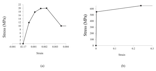
Concrete compressive stress value at ultimate strain depends on the level of confinement and on the axial load. The exact crushing stress due to flexure can be obtained from section analysis hence a lower stress value was used to account for all possibilities and to eliminate numerical instability problems. In addition, modelling of the tensile properties of concrete is neglected since their effect at high seismic excitation levels is regarded as minimal.
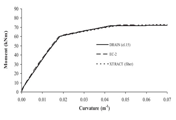
3.2. Moment-Curvature Relationships
To verify the effectiveness of the section discretization described in the previous section, the moment-curvature results obtained by DRAIN-3D for the corresponding column section are compared to results given by a widely used fibre section analysis software XTRACT [21] and manual section analysis calculations based on EC-2 models. The cross-section characteristics are as shown in Fig. (9). The curves show exact agreement with DRAIN-3D Fig. (11), which verifies the accuracy of the section analysis element in DRAIN-3D in predicting member flexural response.
3.3. Modelling Slip Deformations
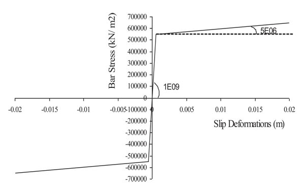
Slip deformations can be incorporated in the nonlinear analysis by connection hinges at element ends, which are available in element 15 of Drain 3dx. These hinges are used to model both the pullout and gap effects and are defined by fibres. These hinges are located at the element ends, where the steel fibers are replaced by pullout fibres and the concrete ones by gap fibres. Based on the experimental results of the Saclay test, the softening effects were activated after the yielding of the main reinforcement, and contributed to additional deformations and that is why connection hinges were included in the numerical model.
Low strength concrete bond strength model [22] for deformed bar and the experimental findings of the strain distribution were used to model the bond–slip (τ-s) behaviour. To evaluate the initial bond stiffness and calculate the elastic slip, a uniform strain distribution was assumed along the embedment length. For the post yield case, a linear strain distribution was assumed to evaluate the plastic slip. In this case, the bond stress value was taken as the residual bond strength for deformed bar in pullout mode, equal to 5.4MPa as calculated using the anchorage capacity model in [14]. The value of the residual slip was used to define the saturated slip for the pullout hinge and this is related to a slip before complete debonding. This residual slip controls the rate of strength degradation of the connection hinge. The resulting backbone curve is shown in Fig. (12). The model is completed by applying the hysteretic rules for the simulation of degradation in loading and unloading cycles. Based on the findings of the strain analysis no strength degradation below fy is applied in the model since the yield strength was achieved. Unloading stiffness is set equal to the initial stiffness based on [23] and cyclic bond model whereas full pinching degradation is assumed in the unloading curve based on findings from cyclic experimental pullout tests conducted by different researchers [22], In addition, unloading stiffness and pinching behavior is consistent with cyclic bond models derived by various researchers [24-27].
3.4. Modelling of Joints
Joints are modelled using a combination of a linear element to account for the elastic joint deformations, and a nonlinear shear element (code name in DRAIN is element 8), to account for additional shear deformations. Element 8 has shear hinges distributed along the element length. These hinges account for additional elastic and inelastic shear deformations. The inelastic shear model in Drain 3dx is used in parallel to a linear elastic model accounting for the elastic flexural deformations prior to the attainment of the shear capacity. There can be up to two shear hinges, for shear deformations in the two local axes. The calibration of the model requires the definition of the shear capacity values and the corresponding elastic and post elastic stiffness. The joint is modelled to behave linear elastically with stiffness equal to EIcr up to the attainment of its shear capacity. In the case of the Saclay frame E=29GPa and Icr=0.5*Ig=0.0019. Elastic shear deformations in this joint are modelled using the cracked shear stiffness
 of the column (Fig. 13).
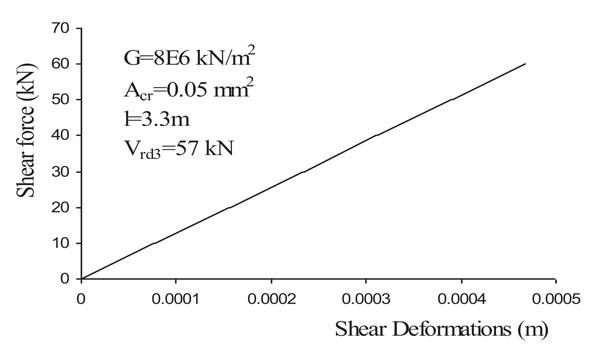
Since the shear column capacity (Vrd3) is higher than the shear force demand observed in [1], which is around 150kN for 4 columns, the shear model is calibrated only for elastic response. The effectiveness of the above mentioned non-linear local element models to simulate the behaviour of the frame was proven in more detail in [1, 3] and [16] through the comparison of both forces and displacement histories.
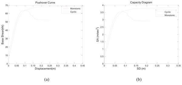
The monotonic and cyclic displacement-based analysis was used to derive the pushover curve of the frame shown in Fig. 14a and b. A constant displacement step was applied for the cyclic analysis and the strength degradation is obvious from the resulting curve since the cyclic behaviour of the anchorage model allows for such. In effect, the cyclic curve is obtained from a number of reversed push-over analyses at controlled increasing displacement demands. Using the equivalent linear SDOF system approximation, this curve is transformed to a capacity curve as defined in the context of capacity demand diagram methods. The capacity curve is used in the following section to evaluate its performance of the frame.
4. SEISMIC DEMAND EVALUATION USING FEMA 440 (IMPROVED NON-LINEAR STATIC METHOD)
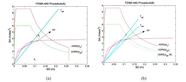
The latest attempt to improve the accuracy of the ATC-40 capacity spectrum method is included in [5] with an improved equivalent linearization procedure, which is still an iterative procedure. The displacement response of the nonlinear SDOF system is computed using an “equivalent” linear system with effective period Teff and damping βeff, which are computed as a function of the ductility demand. Teff varies between initial period To and the secant period Tsec and is generally shorter than Tsec. The two procedures (A and B), adopted in [5] for Performance Point (PP) evaluation, are described below.
- A representative elastic spectrum is selected which is denoted as ADRS (β0) in Fig. (15a).
- PP in Fig. (10a) needs to be assumed in the first iteration on the capacity envelope similar to other CDDM methods and the ductility is calculated through a bilinear force-displacement relation of the idealized SDOF system.
- Teff and βeff for this particular ductility level are calculated by using the equations given in sections 6.2.1 and 6.2.2 of [5] for different ductility ranges.
- The evaluated βeff is substituted into a suitable reduction factor equation given by the procedure in [5], which is used in calculating the highly damped demand spectrum corresponding to βeff from the elastic demand spectrum with viscous damping βo in ADRS format.
- According to procedure A, the maximum displacement di and acceleration ai can be estimated at the intersection of the radial line corresponding to Teff with the demand spectrum (βeff) in ADRS format as shown in Fig. (15a). If these values are within the acceptable tolerance, they are considered as PP. Otherwise iterations are needed until convergence is achieved.
- According to procedure B, only the ADRS (βeff) spectral acceleration ordinate is multiplied by the modification factor
 to develop the Modified Acceleration-Displacement Response Spectrum, MADRS (βeff, M), as shown in Fig. (15b). The modification factor shows the difference in ductility between the equivalent SDOF systems with Tsec and Teff.
The PP is evaluated at the intersection of MADRS (βeff, M) with the capacity envelope. If the estimated PP is within acceptable tolerance with the assumed one then it is regarded as the adopted value. Otherwise, iterations are needed until convergence is achieved. The PP evaluation for the Saclay frame at 0.3g is shown in Figs. (15a, b).
The inclusion of both the damping level (step 4) and the ductility demand level (step 2) to account for nonlinearity at the assumed PP (rather than one of the two) is the unique feature of this capacity demand diagram method.
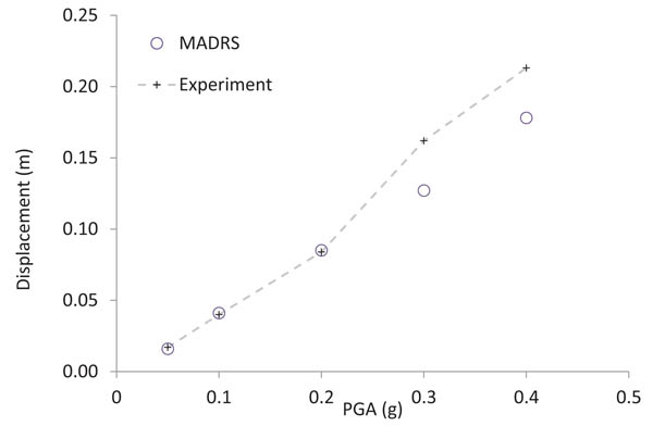
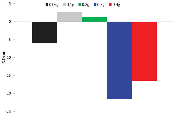
4.1. Performance Point (PP) Prediction Using FEMA 440
The PP predictions for the Saclay frame (at different PGA levels) using the MADRS are compared with experimental displacement demands as shown in Fig. (16). The assumption of elastic perfectly plastic (EPP) appears to be reasonable for the FEMA440 method until 0.2g. However, large under-predictions are observed at higher PGA levels (0.3g and 0.4g, (Fig. 17). As it was shown [1, 3], this change in the behaviour can be attributed to the slip of the reinforcement bars at the column-joint interface causing strength degradation. This suggests the need to investigate other hysteretic behaviour to reduce the error. In this regard, additional hysteretic behaviours other than EPP are examined to assess the best possible seismic demand predictions at higher PGA levels.
4.2. Examination of Different Hysteretic Behaviours Using FEMA (440), MADRS
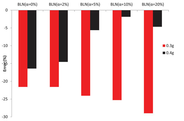
The coefficient values for βeff and Teff proposed in [5] are used to examine different hysteretic behaviour models. These coefficient values correspond to different α-values (α=0% corresponds to EPP behaviour) of a particular hysteretic behaviour.
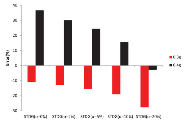
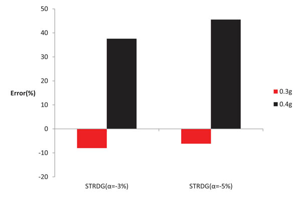
Various hysteretic behaviours such as bilinear (BLN), stiffness degradation (STDG), and strength degradation, (STRDG) were used to assess the best possible one for the Eco-leader building at 0.3g and 0.4g.
For BLN behaviour, the error increases with an increase in α value at 0.3g. BLN with α=0% (EPP) and α=2% gave least error at 0.3g as shown in Fig. (18). For 0.4g, this trend is reversed, and error is minimum at BLN α=10%. Using STDG hysteretic behaviour, the error is minimum for α=0% at 0.3g, whereas at 0.4g, the error is minimum at α=20% as shown in Fig. (19). In general, this hysteretic behaviour is found to be un-conservative for α=0% to 10% at 0.4g. When STRDG hysteretic behaviour is used, the similar trend as STDG is found at both negative α values, but the underestimation is reduced at 0.3g as shown in Fig. (20).
Due to uncertainty related to the choice of the hysteretic behaviour for the substandard structures, a more reliable procedure is required to further refine the seismic demand prediction. The analysis described above includes the monotonic pushover curve which is more suitable for structures subjected to very short duration earthquakes. To account for the cyclic effect of the longer duration earthquake, cyclic-displacements based analysis is carried out to generate capacity curves which account for the degrading effect of the substandard structures. In particular, cyclic displacements account for strength and stiffness degradation due to brittle failure modes such as shear, bond failures and even buckling failure of the main reinforcement bars. These modes of failure are very common in substandard seismic designed structures due to insufficient design code provisions and very poor seismic resistant detailing. In particular, the inadequate bond and lap lengths and the large spacing of shear links are the most common deficiencies that cause degradation when cyclic loading is applied on a substandard structure.
The following section describes a newly developed procedure to model the complex degrading behaviour of the poor quality / substandard structures for the seismic demand evaluation. The analytical models used for the simulation of the above-mentioned failure modes are explained in detail in [1, 3]. Moreover, the seismic performance predictions of case study structures using the cyclic capacity curves and the chosen methodology are also presented.
5. MODELLING COMPLEX DEGRADATION BEHAVIOUR OF NON-DUCTILE EQUIVALENT SYSTEMS
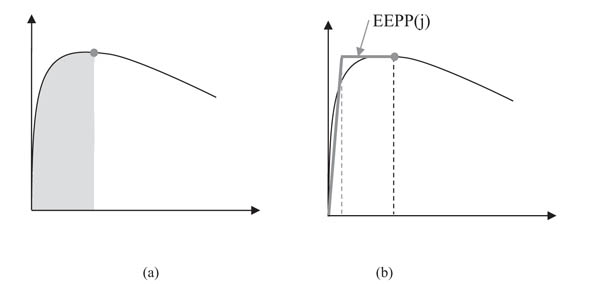
The procedure for the determination of the displacement performance (performance point, PP) using the FEMA440 idealisation procedure [5] was illustrated in the previous section with an application using test results. The conclusions drawn from the comparison of the predictions to the experimental results is that, in this case of a strength degrading system, a considerable error in prediction exists regardless of the hysteretic type and a-value used. This is due to the fact that the idealisation of the capacity curve into a bilinear one cannot capture the true characteristics of the degrading capacity curve of the system i.e. the energy balance between the actual and the idealised capacity curve differs considerably at all points on the curve. In order to assess the detailed characteristics (µ, Tsec) of the capacity curve especially in the case of degrading curves, a reverse procedure is proposed for the idealisation of degrading capacity curves in, which each point (SAi and SDi) on the curve can be considered as a PP. Each PP is assumed to correspond to an Equivalent Elastic Perfectly Plastic system (EEPP) as shown in Fig. (21b). The unrecoverable energy above each PP is ignored (Fig. 21b) and the energy balance between the actual curve and the EEPP system at the specific PP is used to define the initial period, the secant period to the PP and the ductility μ of the EEPP system. This proposed idealisation procedure for degrading capacity curves can be implemented in the context of any capacity demand diagram method. In the following section the proposed procedure will be illustrated using the FEMA440 (MADRS) idealisation procedure.
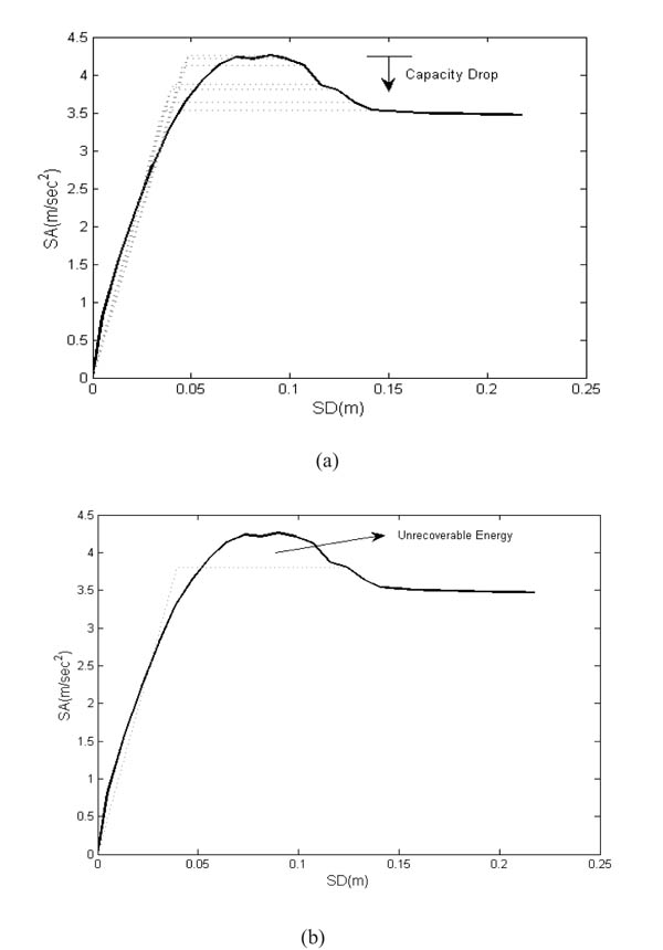
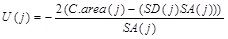
Fig. (22a) shows the cumulative area (c.area (j) under the capacity curve at a SD(j) corresponding to the maximum capacity point. EEPP corresponding to this point is shown in Fig. (22b). Equal area rule (eq.1) is applied and the yield displacement U (j) (eq.2) is obtained by rearranging eq.1.
 |
(1) |
 |
(2) |
The ductility at each PP is evaluated using eq. 3. These ductility values are used to evaluate βeff and Teff using FEMA440 relations. These ductility values are thus used in the iterative process to evaluate seismic demand.
 |
(3) |
6. PERFORMANCE ASSESSMENT OF PROPOSED METHOD (FEMA (EEPP))
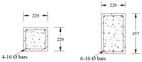
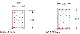
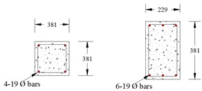
The performance of the proposed EEPP system procedure is assessed by predicting the seismic demand of substandard degrading structures. For this purpose, a simulation study is conducted in which different building categories typically found in the developing countries are analysed for seismic demand evaluation using MADRS and the proposed EEPP procedures. These buildings include further to the Saclay frame, a 2 storey 2 bay building, a 3 storey 3 bay building and a 5 storey 4 bay building. The section details of the buildings (excluding details of the Saclay frame given earlier), are given in Table 4.
| Building Category | Sections | |
|---|---|---|
| Column | Beam | |
| 2 storey 2 bay building (storey height = 2.9 m and bay = 4x4 m) |
 |
|
| 3storey 3 bay building (storey height = 2.9 m and bay = 4x4 m) |
 |
|
| 5 storey 4 bay building (storey height = 2.9 m and bay = 4x4 m) |
 |
|
Ten different models are further generated for each building category from the probabilistic data of key capacity parameters obtained using the Latin Hypercube Sampling (LHS) procedure. Values of different key parameters (f'c, fy, Vn, fs) considered for the analysis of the case structures is given in Table (5) (where = concrete compressive strength, fy = steel yield strength, Vn= shear capacity, fs = bar stress that can occur because of the development length). For more realistic in-elastic analysis of the substandard building models using Drain 3dx, the low strength concrete stress-strain model [17] is used.
| Material Strength | ||||
|---|---|---|---|---|
| Number of Simulation | fc | fy | Vn | fs |
| MPa | MPa | MPa | MPa | |
| 1 | 23 | 382 | 49 | 163 |
| 2 | 24 | 453 | 47 | 314 |
| 3 | 28 | 440 | 44 | 233 |
| 4 | 14 | 477 | 46 | 245 |
| 5 | 18 | 473 | 47 | 335 |
| 6 | 20 | 483 | 47 | 278 |
| 7 | 26 | 409 | 45 | 248 |
| 8 | 16 | 469 | 50 | 144 |
| 9 | 19 | 521 | 48 | 232 |
| 10 | 18 | 485 | 50 | 203 |
Moreover, for introducing reliable bar stress-slip behaviour in the numerical models, the bond-slip characteristics for deformed bar in low strength concrete [22] are used. Hence the structures with these capacity values have different strength and stiffness degradation characteristics. In addition to the above-mentioned parameters, the possible presence of degradation of mechanical characteristics of the materials due to the corrosion effects, cover spalling, buckling of bars also contributes in the strength and stiffness degradation of sub-standard RC structures and components [29]. These effects may also be included in the analysis if the structural material has these deficiencies and based on the sophistication and detail of test results that need to be obtained on corroded steel bars.
Time-history analysis (THA) was carried out using the acceleration record of 0.3g for all buildings except the Saclay frame for which the 0.4g record is used. The maximum displacement from the THA is compared with the predictions of the MADRS and EEPP idealisation procedures to assess the error in demand prediction. The seismic performance predictions obtained using monotonic capacity curves with no strength degradation (MADRS procedure) are compared with the predictions of the EEPP procedure when strength degradation is included in the capacity curves. The strength degradation in the hysteretic response was applied through cyclic-displacements push-over analysis.
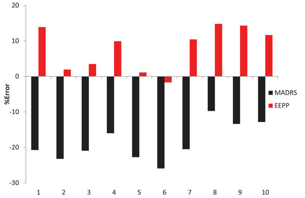
The error in seismic performance predictions using the MADRS (monotonic pushover analysis) and using the proposed EEPP method (cyclic-displacements pushover analysis) for each building category is shown in Figs. (23 and (24a, 24c), Table 6 summarises these results.
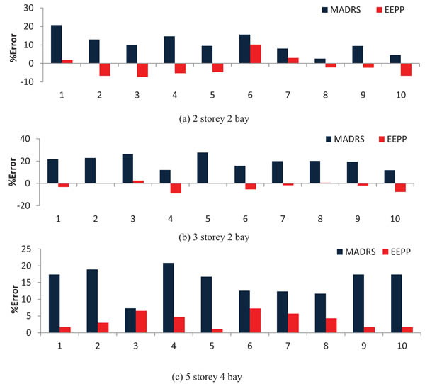
| No | Building | Error (MADRS) | Error (MADRS) | Error (EEPP) | Error (EEPP) |
|---|---|---|---|---|---|
| % (mean) | % (standard deviation.) | % (mean) | % (standard deviation.) | ||
| 1 | Ecoleader | 18.6 | 5.3 | 8.3 | 5.7 |
| 2 | 2st.2bay | 16.4 | 5.3 | 5.8 | 4.1 |
| 3 | 3st.3bay | 19.7 | 5.4 | 3.2 | 3.1 |
| 4 | 5st.4bay | 15.2 | 4.1 | 3.7 | 2.3 |
Based on the results shown in Table 6, it is clear that the EEPP procedure gives better estimation of the structural response than MADRS.
A relatively medium duration time history record was used in the above simulation study. This record was adopted since it resembles the expected seismic activity in the majority of the European region. To further investigate the performance of the proposed EEPP procedure for structures subjected to longer duration earthquakes, an artificial time history record was generated using the SIMQKE program in Shake 2000 [28]. The UBC [30] target spectrum corresponding to the stiff soil (zone 3 and type-A source distance > 10km) was selected. The PGA value of the generated time history is 0.4g and the duration is 60 seconds. Only the 2 story 2 bay structures were selected for this study. The same cycle step (0.3% drift) is adopted as in the previous study. Fig. (25) shows the prediction errors for MADRS and MADRS with modified EEPP.
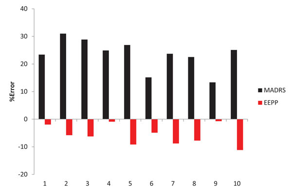
The mean error of MADRS idealisation procedure compared to the exact result from the THA is 23.48% which is much higher than before. The mean error of the proposed EEPP procedure in predicting the THA results is 5.7% and the standard deviation is 3.63% which is almost the same as predicted for 0.3g PGA (Fig. 20). Considering the good performance of the proposed EEPP procedure in predicting the seismic demand of degrading structures in both short and long duration earthquakes, it is suggested that it can be adopted particularly for seismic assessment of existing sub-standard / brittle RC structures typically found in developing countries.
7. DISCUSSION AND CONCLUSION
The non-linear seismic performance prediction of structures using static methods is possible with the use of capacity demand diagram methods, initiated in the late 1990’s as a simple and time effective alternative to complicated time-history analysis. Many such methods exist in the literature differing in the way of accounting for the non-linearity of the structure. These methods have been proven to provide accurate predictions compared to time-history analysis for non-degrading structures with nearly bilinear capacity curves and flexural response.
The latest version of these methods, included in [5], also accounts for a small decrease in the post-peak part of the capacity curve to account for low levels of strength degradation. However, the use of a single small-negative post-peak gradient in the capacity curve has been proven in the present study to provide insignificant improvement in the performance prediction of degrading RC structures mainly since non-ductile modes of failure may result to abrupt reduction of strength (sudden shear failure of column) to a more moderate reduction occurring for example due to the slip of reinforcement in joints. In addition, the post-peak behaviour of strength degrading systems may also include a small non-degrading part prior to the degrading one i.e. exhibit minor flexural behaviour in the post-peak region. Thus, in the case of strength degrading systems a single idealisation procedure may lead to a significant underestimation of the energy under the original response curve.
Based on the above findings, the present study examined an alternative procedure for the idealisation of strength degrading systems which can be used in the context of any capacity demand diagram method. The resulting procedure is based on the discretisation of the capacity curve and the assumption that each point on the curve is a Performance Point (PP), as defined in the capacity diagram methods. Based on this assumption, an EEPP system is plotted for each point on the curve by using the corresponding area to the point under the original curve. Any capacity demand diagram method can be applied backwards to estimate the corresponding PGA related to each PP. The procedure can be extended by correlating the PP’s to displacement related damage levels in order to obtain a curve of the evolution of damage with the increase in PGA. The proposed procedure was compared herein to the original idealisation procedure in [5] and has proven to provide improved performance predictions when compared with experimental results. The comparison was conducted in a small probabilistic case study and needs to be extended to account for larger structures. Integrating the proposed idealisation procedure with MADRS [5], led to reduced prediction error of time-history analysis results compared to using MADRS as proposed in [5]. It should be noted that the simplification proposed herein for performance prediction can be proven very efficient for fragility curve derivation studies such as [31] by eliminating the need of cumbersome time-history analyses.
The case study was applied to a frame structure with good correlation, but needs to be extended to other structural systems such as a RC frame strengthened with RC Infill walls [32] for which pseudo-dynamic test results are available.
LIST OF ABBREVIATIONS
| ADRS | = Acceleration Displacement Response Spectrum |
| BLN | = Bilinear |
| CDDM | = Capacity Demand Diagram Methods |
| DCM | = Displacement Coefficient Method |
| EP | = Elastic-Plastic |
| EPP | = Elastic Perfectly Plastic |
| EEPP | = Equivalent Elastic Perfectly Plastic |
| GLD | = Gravity Loaded Design |
| LSC | = Low Strength Concrete |
| MADRS | = Modified Acceleration Displacement Response Spectrum |
| MDOF | = Multi Degree of Freedom |
| NSM | = Non-Linear Static Method |
| NERC | = Non-Engineered Reinforced Concrete |
| PGA | = Peak Ground Acceleration |
| RC | = Reinforced Concrete |
| SA | = Spectral Acceleration |
| SD | = Spectral Displacement |
| SDOF | = Single Degree of Freedom |
| STDG | = Stiffness Degradation |
| STRDG | = Strength Degradation |
| THA | = Time History Analysis |
| fcmax, f'c | = Concrete compressive strength |
| fy | = Steel bar yield strength |
| Teff | = Effective period |
| Teq | = Equivalent period |
| Tc | = Upper limit for the period of the constant spectral acceleration branch |
| Tsec | = Secant period |
| α | = Gradient of degrading part of capacity curve |
| βeff | = Effective damping |
| βeq | = ξeq Equivalent damping |
| λ | = Correction factor |
| µ | = Ductility ratio |
| τmax | = τe bond strength for elastic steel |
CONSENT FOR PUBLICATION
Not applicable.
CONFLICT OF INTEREST
The authors declare no conflict of interest, financial or otherwise.
The research work of the first author is supported by the Overseas Research Student (ORS) award scheme of the Vice-Chancellors’ committee of the United Kingdom’s universities. Second author research is supported by Higher Education Commission (HEC), Pakistan
ACKNOWLEDGEMENTS
The authors wish to acknowledge the technical and financial assistance offered by the Centre for Cement and Concrete of the University of Sheffield. The first author also acknowledges the financial support provided by the Overseas Research Student (ORS) award scheme of the Vice-Chancellors’ committee of the United Kingdom’s universities as well as the A.G. Leventis Foundation. In addition, the second author acknowledges the financial support provided by Higher Education Commission (HEC), Pakistan to conduct this research as a part of developing analytical seismic vulnerability assessment framework for reinforced concrete structures of developing countries.