All published articles of this journal are available on ScienceDirect.

An Artificial Neural Network Model for Predicting the Maximum Allowable Heat Release of Concrete during the Construction of Massive Monolithic Foundation Slabs
Abstract
Introduction
Early-age cracking in mass concrete structures, driven by thermal stresses from cement hydration, remains a critical durability concern. One effective way to reduce the risk of early cracking is to select a concrete mixture formulation that reduces heat emission. This study considers, for the first time, the inverse problem of preventing early crack formation: determining the maximum allowable concrete heat release (Qmax) for the given geometric characteristics of the structure and concreting parameters using machine learning methods.
Materials and Methods
A dataset of 39,200 numerical experiments was collected via thermo-mechanical modeling, considering variables like slab thickness, heat transfer coefficient, concrete grade, ambient temperature, and concreting duration. The target value Qmax was identified using the bisection method, ensuring the tensile stress-to-strength ratio remained below unity. A feedforward Artificial Neural Network (ANN) with two hidden layers was developed and trained on this dataset.
Results
The ANN model achieved exceptional prediction accuracy, with a correlation coefficient of 0.99955 between target and predicted Qmax values. Analysis revealed that the concrete compressive strength grade had a minimal effect on the maximum permissible heat release.
Discussion
Feature importance analysis showed that the curing rate and slab thickness are the most significant parameters influencing the Qmax value. The negligible impact of compressive strength stems from its competing effects on tensile strength and elastic modulus.
Conclusion
The developed ANN model provides a highly accurate tool for predicting permissible concrete heat release, enabling optimized mix design to mitigate early thermal cracking in massive foundation slabs.
1. INTRODUCTION
The challenge of early-age cracking in mass monolithic reinforced concrete structures has remained a persistent issue since the inception of reinforced concrete technology in the 19th century [1]. The cracking mechanism is associated with tensile stresses developed in concrete during hardening that exceed its tensile strength [2]. The key factor driving these stresses is a non-uniform temperature field caused by the exothermic heat of cement hydration. Cracks that appeared at the construction stage compromise the structural serviceability, load-bearing capacity, and durability of constructions [3].
A range of technological measures is employed to minimize the risk of early cracking. The use of insulated formwork reduces convective heat exchange between the concrete surface and the environment, thereby mitigating temperature gradients [4]. The method of internal pipe cooling, implemented by circulating a coolant through pipes embedded within the structure, provides controlled heat extraction and homogenization of the temperature field [5]. Introducing chemical admixtures (plasticizers, superplasticizers, set retarders) into the concrete mix allows for the regulation of hydration kinetics, reducing peak temperatures and thermal gradients [6, 7]. Pre-heating the subgrade before concrete placement in freezing conditions reduces the critical thermal gradient at the interface with the cold foundation, thereby enhancing crack resistance [8]. Cement fineness is also a significant parameter: utilizing cements with a lower specific surface area slows the rate of heat release, distributing it over time, which reduces internal stresses without compromising long-term design strength [9].
A fundamental aspect in the design of mass concrete structures is the proportioning of concrete mixes, aimed not only at achieving the required strength but also at ensuring crack resistance during the exothermic heating and subsequent cooling phases [10]. Managing heat generation is achieved by selecting low-heat binders (slag Portland cements, pozzolanic cements, cements with reduced C3A content) and employing supplementary cementitious materials (fly ash, microsilica, metakaolin) to partially replace Portland cement [11-14]. Consequently, high-alumina cements and limestone Portland cements are typically excluded due to their intense and rapid heat release [15, 16]. Using larger aggregate fractions reduces the specific surface area, thereby lowering the required cement paste content and total heat generation while enabling a dense particle packing in the mix [17, 18].
Optimal measures to mitigate the risk of early cracking can be selected based on numerical modeling. The Finite Element Method (FEM) is the primary tool for solving coupled problems of transient heat transfer and stress analysis; however, it is characterized by high sensitivity to input parameters and computational complexity [19, 20]. The finite difference method encounters difficulties when modeling objects with complex geometry [21]. The discrete element method, which models material behavior at the meso-level, demands significant computational resources and complex calibration [22]. Extended FEM techniques (XFEM) and modern non-local methods (peridynamics, phase-field) offer high accuracy in crack modeling but are noted for their implementation complexity and high computational cost [23, 24].
In contrast to algorithmic approaches, machine learning methods, particularly artificial neural networks (ANNs), can uncover hidden nonlinear relationships from empirical data, offering high-speed prediction and potential for concrete mix optimization [25].
All existing models focus on solving the direct problem of predicting temperature fields and stresses. However, for practical design purposes, solution of the inverse problem is critical: determining the maximum permissible level of concrete heat generation (Qmax) that guarantees the absence of thermal cracks during the structure-forming period. Solving the inverse problem using direct modeling (e.g., iteratively fitting Qmax using a full thermomechanical model) requires substantial computational resources and time for each set of input parameters. Trained artificial neural network models can overcome this limitation by providing instant prediction of the required parameters with the highest accuracy after completing the training stage.
This article introduces a novel predictive framework for establishing the maximum allowable heat release (Qmax) in mass concrete foundation slabs. For the first time, a solution is provided to mitigate thermal stress and prevent cracking during the critical hardening phase of monolithic construction. This study changes the paradigm by addressing an inverse problem: what is the maximum concrete heat release (Qmax) acceptable for given geometric and process parameters to ensure a crack-free structure? The crack resistance criterion is defined as the condition in which the ratio of the maximum tensile stress to the tensile strength does not exceed unity. Solving this problem holds substantial practical significance for optimizing concrete mix designs in the construction of mass concrete structures.
2. MATERIALS AND METHODS
The following values were selected as input parameters of the model:
- Thickness of the foundation slab h (m)
- Ambient temperature T∞ (°C)
- Heat transfer coefficient on the upper surface hup (W/(m2 ∙°C))
- Concrete compressive strength grade B (MPa) according to Russian standard GOST 10180-2012
- Time for concreting one layer of the slab tbr (hr)
- Hardening rate.
Unlike our previously developed models [26-27], the variable tbr was introduced to account for the layer-by-layer nature of the concreting process. The layer thickness for all variants was assumed to be 0.25 m when creating the training dataset.
The ranges and step sizes of the input parameters are taken in accordance with Table 1. For a curing rate of 0, this corresponds to slow-hardening concrete, while 1 corresponds to rapid-hardening concrete. A layer concreting time tbr of 0 hours means that the structure is poured in one go.
| Parameter | Lower Limit | Upper Limit | Step |
|---|---|---|---|
| Thickness of the foundation slab h (m) | 0.75 | 3 | 0.25 |
| Ambient temperature T∞ (°C) | 5 | 35 | 5 |
| Heat transfer coefficient on the upper surface hup (W/(m2 ∙°C)) | 2 | 30 | 4 |
| Concrete compressive strength grade B (MPa) | 25 | 45 | 5 |
| Time for concreting one layer tbr (hr) | 0 | 6 | 1 |
| Hardening rate | 0 | 1 | 1 |
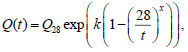
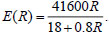
The heat release function was set by the Eq. (1):
 (1)
(1)
where t is the time in days, Q28 is the amount of heat released during the first 28 days of hardening, MJ/m3, and the coefficients k and x depend on the rate of hardening of the concrete.
The value Qmax = Q28 (MJ/m3) was taken as the output variable. The choice of Q28 as a proxy variable for the maximum permissible heat release is motivated by the following. Early thermal cracking in massive concrete typically occurs in the first days and weeks after placement, when the rate of heat release is highest, and the concrete's strength is still low. By 28 days, hydration, especially for conventional cements, is largely complete, and intense heat release ceases. Thus, the total heat released by the 28th day fully characterizes the thermal “load” that leads to stress development during the critical early period.
From Equation 1, it can be seen that the parameter Q28 is a scaling coefficient that determines the overall scale of the heat release curve Q(t). For fixed kinetic parameters k and x, an increase in Q28 leads to a proportional increase in heat release at any time t, including the peak period. Therefore, monitoring Q28 is equivalent to monitoring the entire time dependence of Q(t) in the context of assessing peak temperatures and gradients.
For each data sample [h hupT∞B rate tbr] the determination of the maximum permissible heat release value Qmax = Q28 was performed using the bisection method. A value of Q28 was found in the range from 20 to 520 MJ/m3 at which the maximum tensile stress level (the ratio of tensile stress to current tensile strength σ/Rt) was equal to one. The permissible error in finding the value of Qmax using the bisection method was assumed to be 1%.
The stress level was determined using a methodology validated against experimental data and presented in the paper [28]. A comparison with experimental data is not presented here, as it was previously performed in papers [26, 27, 29]. The thermophysical properties of the soil were not included in the input parameters for constructing the machine learning model. This is supported by a previous study [26], which showed that their influence on stress levels is not very significant, averaging less than 5%. Numerical calculations for constructing the training dataset were performed for the following values of the soil's thermophysical properties: density ρg = 2000 kg/m3, thermal conductivity λg = 1.62 W/(m · °C), and specific heat capacity of the soil cg = 2250 J/(kg · °C). Other constant parameters of the model are given in Table 2.
| Parameter | Units of Measurement | Value |
|---|---|---|
| Poisson's ratio of concrete | - | 0.2 |
| Density of concrete | kg/m3 | 2400 |
| Specific heat capacity of concrete | J/(kg∙°C) | 1000 |
| Thermal conductivity coefficient of concrete | W/(m∙°С) | 2.67 |
| Thickness of the soil massif | m | 3 |
| Coefficient of linear thermal expansion of concrete | 1/°C | 10 -5 |
| Time step in calculating the thermal stress state | hr | 0.1 |
| Number of finite elements across the plate thickness | - | 40 |
| Number of finite elements by thickness of soil massif | - | 40 |
The initial temperature of the concrete mixture T0 was assumed to depend on the ambient temperature and was determined by Eq. (2):
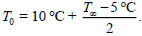 (2)
(2)
The compressive strength of concrete was determined as a function of its degree of maturity using the Eq. (3) [28]:
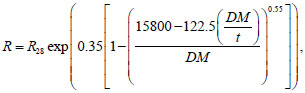 (3)
(3)
where R28 = B + 12 is the compressive strength at the design age of 28 days (MPa), t is the time in hours, DM is the degree of maturity of concrete, determined by the integral (Eq. 4):
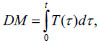 (4)
(4)
where T(τ) is the concrete temperature at the age τ.
The modulus of elasticity of concrete and its tensile strength were related to its compressive strength. For the modulus of elasticity, Karpenko's [30] Eq. (5) was used:
 (5)
(5)
For tensile strength, the formula of Nesvetaev et al. [31] was used (Eq. 6):
 (6)
(6)
Accepted values of parameters k and x in Eq. (1) for rapid-hardening and slow-hardening concrete are given in Table 3.
| - | - | k | x |
|---|---|---|---|
| Quick-hardening | - | 0.145 | 0.485 |
| Slow-hardening | - | 0.27 | 0.715 |
The flowchart for the formation of the training dataset is shown in Fig. (1). σ in this figure is the tensile stress.
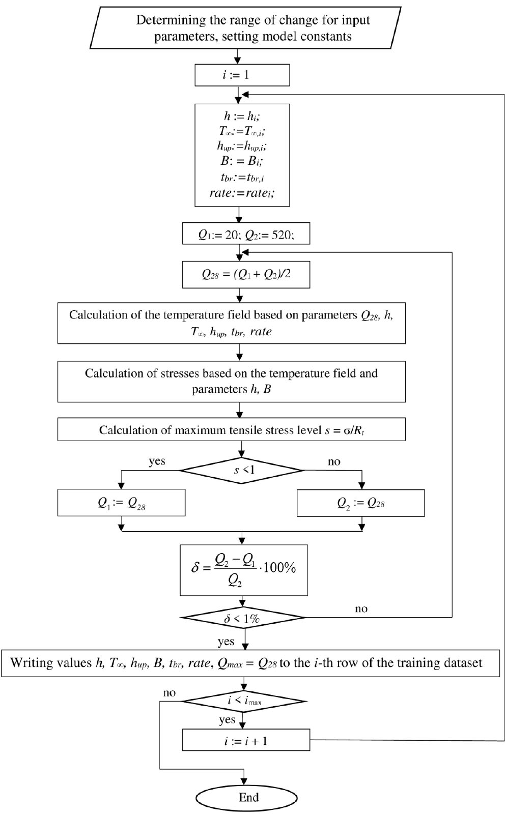
Flowchart of training dataset formation.
Table 4 partially presents the resulting dataset for training the artificial intelligence model. The download link is in the “Data Availability Statement” section. The total training dataset size consisted of 39,200 numerical experiments. Note that the identical Qmax value in this dataset, 518.05 MJ/m3, indicates that the upper limit of the maximum permissible heat release was reached with an error of 1%. With such initial data, the problem of early cracking does not arise. The statistical characteristics of the input and output parameters are presented in Table 5.
| No. | h (m) | T∞ (°C) | hup (W/(m2 ⋅ °C)) | B (MPa) | Rate | tbr (hr) | Qmax (MJ/m3) |
|---|---|---|---|---|---|---|---|
| 1 | 0.75 | 2 | 5 | 25 | 0 | 0 | 518.05 |
| 2 | 0.75 | 2 | 5 | 25 | 0 | 1 | 518.05 |
| 3 | 0.75 | 2 | 5 | 25 | 0 | 2 | 518.05 |
| 4 | 0.75 | 2 | 5 | 25 | 0 | 3 | 518.05 |
| 5 | 0.75 | 2 | 5 | 25 | 0 | 4 | 502.42 |
| 6 | 0.75 | 2 | 5 | 25 | 0 | 5 | 478.98 |
| 7 | 0.75 | 2 | 5 | 25 | 0 | 6 | 455.55 |
| 8 | 0.75 | 2 | 5 | 25 | 1 | 0 | 384.26 |
| 9 | 0.75 | 2 | 5 | 25 | 1 | 1 | 366.68 |
| … | … | … | … | … | … | … | … |
| 39193 | 3 | 30 | 35 | 45 | 0 | 6 | 90.07 |
| 39194 | 3 | 30 | 35 | 45 | 1 | 0 | 72.00 |
| 39195 | 3 | 30 | 35 | 45 | 1 | 1 | 81.77 |
| 39196 | 3 | 30 | 35 | 45 | 1 | 2 | 94.95 |
| 39197 | 3 | 30 | 35 | 45 | 1 | 3 | 94.95 |
| 39198 | 3 | 30 | 35 | 45 | 1 | 4 | 86.65 |
| 39199 | 3 | 30 | 35 | 45 | 1 | 5 | 80.30 |
| 39200 | 3 | 30 | 35 | 45 | 1 | 6 | 75.42 |
| Parameter | h (m) | T∞ (°C) |
hup (W/(m2∙°С)) |
B (MPa) | Rate | tbr (hr) | Qmax (MJ/m3) |
|---|---|---|---|---|---|---|---|
| Average | 1.875 | 20 | 16 | 35 | 0.5 | 3 | 162.35 |
| Std. dev. | 0.718 | 10 | 9.165 | 7.071 | 0.5 | 2 | 84.3 |
| Min | 0.75 | 5 | 2 | 25 | 0 | 0 | 28.91 |
| 25% | 1.25 | 10 | 8 | 30 | 0 | 1 | 102.52 |
| 50% | 1.875 | 20 | 16 | 35 | 0.5 | 3 | 136.7 |
| 75% | 2.5 | 30 | 24 | 40 | 1 | 5 | 200.66 |
| Max | 3 | 35 | 30 | 45 | 1 | 6 | 518.05 |
A feedforward artificial neural network was chosen as a machine learning method. The input data is a static set of numerical features describing the project's specific conditions. It is not a time series (such as monitoring data over time), a sequence or signal, or data with a spatial structure (such as an image). Therefore, architectures specialized for such data types (e.g., recurrent networks (RNNs) and convolutional networks (CNNs)) are unnecessary and would only complicate the model. The problem involves regression analysis which consists in constructing a nonlinear function mapping a 6-dimensional space of input parameters to a 1-dimensional value of Qmax. Feedforward Neural Networks (FNNs) are universal approximators and are ideal for modeling complex nonlinear relationships between fixed sets of features and the target variable. They are the standard and most effective choice for problems of this type.
The architecture of the neural network used is shown in Fig. (2). The neural network includes 2 hidden layers with 16 neurons each. The dependence of Qmax on the input parameters is not a simple linear or quadratic function. It involves complex thermomechanical relationships described by a system of differential equations. A single hidden layer can, in theory, approximate any continuous function (Tsybenko's theorem), but in practice, complex dependencies may require an exponentially large number of neurons. Two hidden layers allow the network to construct a more hierarchical and efficient internal representation of the data. The first hidden layer can extract primary, relatively simple nonlinear combinations of input parameters (e.g., the interaction between h and hup). The second hidden layer can combine the primary features from the first layer to form more abstract, complex representations necessary for accurate Qmax prediction. A two-layer architecture is a compromise between accuracy and computational complexity. It has significantly greater capacity (approximation ability) than a single-layer network, but remains less complex and more resistant to overfitting than a deep network with three or more layers, which is excessive for six input parameters and the smooth nature of the data.
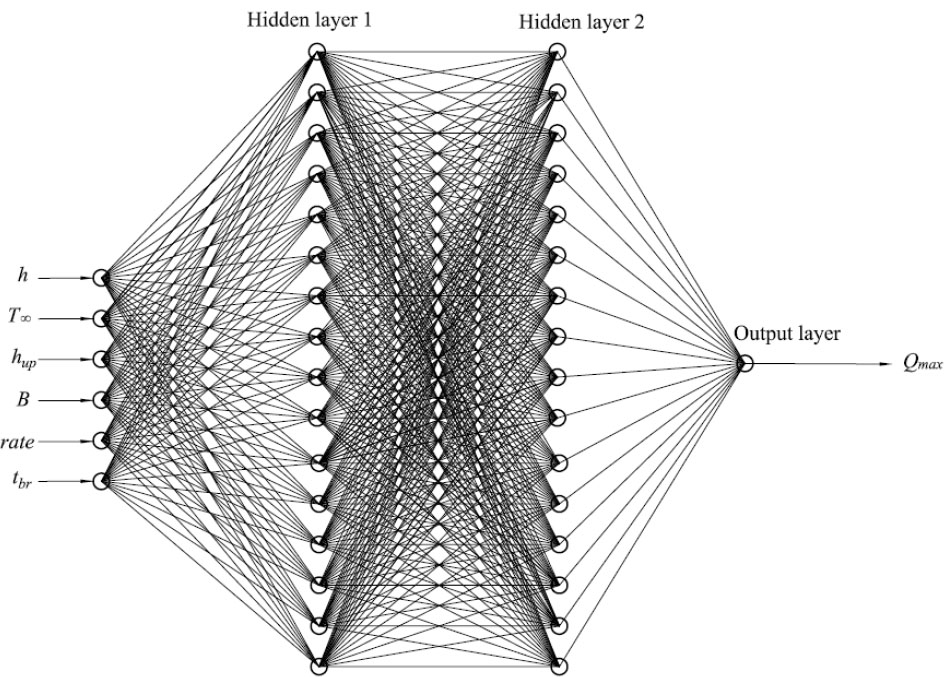
Architecture of an artificial neural network.
Regarding the number of neurons, there are empirical rules relating the number of neurons to the input dimension. The number of neurons is often chosen between the input dimension (6) and the output dimension (1), perhaps 2-3 times greater. A range of 10-20 neurons is typical for problems of this dimension.
TANSIG (hyperbolic tangent) was used as the activation function for neurons. This choice is motivated by its nonlinear, smooth (differentiable), and symmetric nature, yielding values the range (-1, 1). These properties make it particularly suitable for regression problems. The procedure for forming the training dataset and the machine learning model was implemented in MATLAB. For training, the dataset was divided into 3 parts “Train”, ”Validation” and “Test”. The sample size of “Train” was 27440 rows. The sample sizes for “Validation” and “Test” were 5880 rows each. Data normalization was performed before training. Since the synthetic data are highly smooth, smoothing was not required. The Mean Square Error (MSE) was used as a training quality metric. The model was trained using the Levenberg-Marquardt algorithm [32, 33]. The choice of this algorithm was driven by a systematic approach that took into account the size and nature of the data (moderate volume, smoothness), the size of the network (small), and the priority of achieving maximum prediction accuracy.
3. RESULTS
Table 6 presents the correlation coefficients between the input parameters and the output variable Qmax. It also shows that the input variables in the resulting dataset are uncorrelated (orthogonal). This is a direct consequence of the method used to construct synthetic data, which employs a full factorial design in which the values of each parameter vary independently within specified ranges (Table 1). This data structure is optimal for model training, as it allows for the isolated assessment of each factor's influence and prevents multicollinearity. However, in real engineering practice, statistical relationships may exist between some parameters (for example, a higher curing rate may be more often used at lower ambient temperatures or for higher-grade concrete).
| - | h | T∞ | hup | B | Rate | tbr | Qmax |
|---|---|---|---|---|---|---|---|
| h | 1 | 0 | 0 | 0 | 0 | 0 | -0.7946 |
| T∞ | 0 | 1 | 0 | 0 | 0 | 0 | -0.1522 |
| hup | 0 | 0 | 1 | 0 | 0 | 0 | -0.2502 |
| B | 0 | 0 | 0 | 1 | 0 | 0 | 0.0104 |
| rate | 0 | 0 | 0 | 0 | 1 | 0 | 0.0582 |
| tbr | 0 | 0 | 0 | 0 | 0 | 1 | 0.0481 |
| Qmax | -0.7946 | -0.1522 | -0.2502 | 0.0104 | 0.0582 | 0.0481 | 1 |
A strong (|RXY| > 0.7) negative correlation is observed between the foundation slab thickness and the permissible heat release level. A very weak correlation is observed between the remaining input parameters and the Qmax value (|RXY| < 0.3).
Figure 3 shows the progress of the training process. Compared to the work [26], which focused on the direct problem of predicting the risk of early cracking, the architecture of the artificial neural network was more complex: the number of neurons in the hidden layers was increased from 12 to 16. Starting with 12 neurons (as in the previous model for the forward problem), the authors found that solving the more complex inverse problem required a slightly larger model capacity. The use of 16 neurons enabled high-quality prediction. The training process took 195 iterations, and the best value of the root-mean-square error was 6.94 MJ2/m6 at iteration 189. The lines corresponding to the “Train”, “Validation”, and “Test” samples are located very close to each other, indicating their representativeness and sufficient volume. The fact that the errors across all three samples are almost identical and have stabilized is the main evidence that the chosen structure (2x16) is neither insufficient (underfitting) nor excessive (overfitting), but is at the point of optimal generalization.
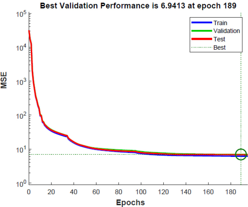
Training performance graph.
The value of MSE equal to 6.94 MJ2/m6 corresponds to the root mean square error (RMSE) equal to √6.94 = 2.63 MJ/m3. The mean Qmax in the dataset is 162.35 MJ/m3, with a range of 28.91 to 518.05 MJ/m3 (Table 5). Relative RMSE error: (2.63/162.35) ∙ 100% ≈ 1.62% of the mean. The error of 2.63 MJ/m3 is extremely small compared to the overall data spread (~490 MJ/m3).
Regression plots for the “Train”, “Validation”, “Test” samples, and the entire dataset (“All”) are presented in Fig. (4). The target values T are plotted on the abscissa axis. The predicted values of permissible heat release, Y, are plotted on the ordinate axis. The correlation coefficient RYT between the target and predicted values for the entire dataset is 0.99955.
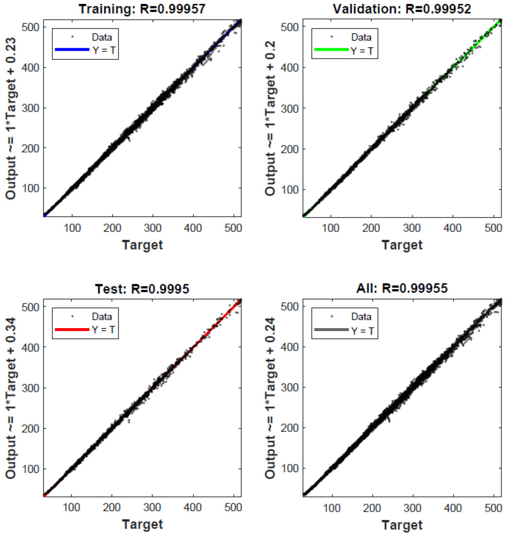
Regression plots for the trained model.
4. DISCUSSION
The correlation coefficient R = 0.99955 between the ANN predictions and the dataset reference values indicates that the ANN's accuracy is virtually identical to that of the original detailed model based on finite element modeling within the training data range. The mean-square error (MSE = 6.94 MJ2/m6) further confirms the high accuracy of the predictions.
| Variable | h(m) | T∞ (°C) | hup (W/(m2∙ °C)) | B (MPa) | Rate | tbr(hr) |
|---|---|---|---|---|---|---|
| Significance Zi (%) | 30.6 | 10 .9 | 8.9 | 0.78 | 70.3 | 11.8 |
Obtaining a solution for a single set of input parameters (h, T∞, hup, B, rate, tbr) requires dozens of bisection iterations. Each iteration is a full-scale FEM calculation of the transient temperature field and stress-strain state, which takes from several minutes to tens of minutes of computational time depending on the mesh detail and model complexity.
After completing the one-time, expensive training and dataset generation phase, the Qmax prediction for a new set of parameters is instantaneous (a fraction of a second). This is orders of magnitude faster than the traditional approach. Thus, ANN shifts the computational burden from the design stage to the pre-training stage, which is a key advantage for practical applications.
The close agreement between the error curves for the training, validation, and test sets (Fig. 3) and the high R values for all sets (Fig. 4) indicate that the model is not overfitted and is highly robust within the studied parameter space. It reliably interpolates results for any combination within these limits.
The obtained correlations between the input and output parameters correspond to the physics and mechanics of the process under study. The strong negative relationship between the foundation slab thickness and the permissible heat release level (RXY = -0.7946) is explained by the fact that increasing the slab thickness reduces its heat dissipation capacity. This leads to large temperature differences between the center and surface of the structure and, consequently, an increase in the maximum tensile stress. Clearly, as the structural bulk increases, the maximum permissible heat dissipation value should decrease.
The weak negative relationship between the parameters hup and Qmax (RXY = -0.2502) can be explained by the fact that a decrease in the heat transfer coefficient on the upper surface results in lower temperature gradients [34]. This well-known technique for regulating heat transfer parameters, successfully applied in [35-37], allows the use of compositions with higher exothermy.
The weak negative relationship between the parameters T∞ and Qmax (RXY = -0.1522) also has an explanation. An increase in ambient temperature raises the maximum temperature within the structure, requiring a reduction in the maximum permissible heat release. This is especially relevant when working in hot climates [38-41].
Regarding concrete grade, an increase in compressive strength is accompanied by an increase in tensile strength, as can be seen, for example, from Eq. (6). An increase in tensile strength allows the structure to better resist thermal tensile stresses. However, an increase in compressive strength is also accompanied by an increase in the modulus of elasticity of the concrete [42], which leads to increased stresses. Therefore, of all the input parameters, concrete grade B demonstrates a minimum correlation coefficient with the value of Qmax (RXY = 0.0104).
The curing rate of concrete has an ambiguous effect on the maximum tensile stress level, as shown in paper [26]. In some cases, rapid-hardening concrete is preferable [43], whereas in others, slow-hardening concrete promotes more favorable temperature conditions and reduces the risk of early cracking [44, 45]. Due to this ambiguous effect on the stress level, the correlation coefficient between the rate and Qmax parameters is close to zero (RXY = 0.0582). The same applies to the layer concreting duration parameter tbr, which also shows a low correlation with Qmax (RXY = 0.481). When using rapid-hardening concrete, the extension of the concreting process over time leads to deterioration in the mechanical performance of the structure, whereas in slow-hardening concrete, an increase in the value of tbr may provide a positive synergistic effect [46].
It should be noted that the correlation coefficient is only suitable for a preliminary assessment of the relationship between variables. Correlation analysis, unlike artificial neural networks, does not allow for capturing complex nonlinear relationships between input and output parameters. Therefore, the feature significance was also assessed using a trained artificial neural network. The significance of features was assessed using the value-fixing method. The results of assessing the significance of input variables in predicting the maximum permissible heat release are presented in Table 7. The Zi value in percent for the i-th feature means that, when calculating Qmax using the average value of the feature across the entire dataset instead of the actual value, the average error will be Zi percent.
Table 7 shows that the most significant parameters are the curing rate and the foundation slab thickness. The remainingceasing importance: tbr, T∞, hup, B. The average effect of concrete grade B on Qmax is no more than 1%, and, therefore, this value can be excluded from the input variables.
5. STUDY LIMITATIONS
- The developed machine learning model can produce reliable results only within the range of input parameters on which it was trained. This range is presented in Table 1.
- The initial temperature of the concrete mix was linked to the ambient temperature Equation 2. The model is not suitable for cases where the temperature of the concrete mix is artificially lowered by adding ice, etc., as occurs, for example, when working in extremely hot climates. To take this factor into account, it is necessary to introduce an additional input parameter to the model, which is a prospect for our further research. Despite this limitation, the adopted assumption allowed us to focus on studying the influence of six key design and process parameters (slab thickness, heat transfer conditions, strength class, curing rate, installation time, and ambient temperature) on the maximum allowable heat release. The model establishes qualitative and quantitative relationships between these parameters and Qmax. It remains adequate for a wide range of scenarios in which the mixture temperature is not actively controlled and instead depends on current weather conditions.
- During the formation of the training dataset, stress levels were determined without accounting for concrete creep. The actual stress level, when creep is considered, will be lower than the calculated value. Consequently, the developed model predicts the permissible heat release level with a certain safety margin. Future research could focus on enhancing the model by integrating creep parameters.
CONCLUSION
This study successfully developed an artificial neural network model capable of predicting the maximum allowable heat release for massive monolithic foundation slabs with exceptional accuracy (R = 0.99955, MSE = 6.94 MJ2/m6), solving this inverse problem for the first time. Based on a comprehensive dataset of 39,200 numerical experiments, the model identified concrete curing rate and slab thickness as the most significant factors influencing permissible heat release, while revealing that concrete compressive strength grade has a negligible impact (less than 1% significance) and can be omitted from the input parameters without compromising prediction accuracy. The developed tool enables engineers to obtain instantaneous, highly reliable estimates of permissible concrete heat release during the design stage, facilitating informed decisions on concrete mix composition to mitigate early-age thermal cracking in massive structures. The final confirmation of the model's practical value will be its validation using data from real projects, where the actual concrete placement parameters and mix composition are known, and the absence (or presence) of cracks has been confirmed. This validation phase is a logical next step in this research's development. Implementing the model as a software module or a web tool with a user-friendly interface will enable the accumulation of such data for continuous model improvement and updates.
AUTHORS’ CONTRIBUTIONS
The authors confirm contribution to the paper as follows: A.C.: Conceived and designed the study; V.T.: Developed software and conducted analysis; D.T.: Drafted the manuscript. All authors reviewed the results and approved the final version of the manuscript.
LIST OF ABBREVIATIONS
| FEM | = Finite Element Method |
| XFEM | = Extended Finite Element Method |
| ANN | = Artificial Neural Network |
AVAILABILITY OF DATA AND MATERIALS
The training dataset is available for download at the link: https://disk.yandex.ru/i/SC8wXh1uhGpSbg.
FUNDING
The study was supported by the grant of the Russian Science Foundation No. 25-19-00164, https://rscf.ru/ project/25-19-00164/.
ACKNOWLEDGEMENTS
The authors would like to acknowledge the administration of Don State Technical University, Russia, for its resources, and the Russian Science Foundation for its financial support.