All published articles of this journal are available on ScienceDirect.

Asymmetric Folded Plate with Parallel Edges in Validation of their Static Behavior by Combining Vlasov Torsion Theory with Bernoulli Bending Theory
Authors Info & Affiliations
Abstract
Aims:
A new hybrid procedure that combines the Vlasov torsion theory with the Bernoulli bending theory is presented herein, to demonstrate qualitatively and quantitatively the operation of asymmetric folded plates with parallel edges, which are loaded with gravity static loads.
Background:
A recently proposed technique based on Vlasov torsion theory is used for the exact calculation of the Principal Elastic Reference System in a reinforced concrete folded plate having an asymmetric thin-walled open cross-section with parallel edges. Moreover, the warping moment (or bi-moment) concept of the Vlasov theory is combined with the pure-bending around two axes, according to the Bernoulli bending theory, to determine the normal stresses along the longitudinal dimension of the folded plate.
Methods:
Τhe warping properties of a thin-walled open cross-section are determined by calculating: (a) the elastic characteristics (elastic center, principal axes) of the section, (b) the principal start point, the sectorial coordinates, the wrapping moment of inertia and the wrapping stiffness of the section. Finally, the normal stresses along the longitudinal dimension are calculated considering the bi-axes flexure with the bi-moment phenomenon.
Results:
Τhe exact solution of normal stresses at the middle section of an examined folded plate along the longitudinal dimension is found by combining the Bernoulli bending theory for prismatic beams and the Vlasov torsion theory for thin-walled open sections.
Conclusion:
The current procedure can be used as a benchmark analysis method of asymmetric folded plates in order to evaluate the reliability of the results of various analysis F.E.M. software, covering an open issue of the structural analysis of special structures.
1. INTRODUCTION
A structural member with a thin-walled open cross-section is often used as a core in multi-story reinforced concrete (RC) buildings or as a roof in folded plate RC structures. In the general case, this cross-section is asymmetric, having strongly spatial behavior that significantly affects the torsional-translational behavior of the structure. Examples of the use of open cross sections are folded plates loaded with gravity loads that are used as roofs, especially in structures with large spans, as well as vertical cores that are usually used in buildings to carry lateral loads (such as seismic or wind loads). The elastic center of the asymmetric cross-section is generally located away from its geometric center and this distance is called “cross sectional eccentricity”. Due to the existence of the partial legs of the thin wall cross-section, the thin-wall open cross-section presents important translational stiffness and significant resistance in bend-from-torsion (phenomenon of torsion-warping).
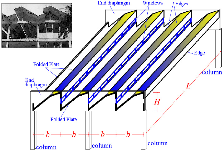
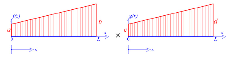
A folded plate consists of -plane surface disks that are not the same, which are connected, as shown in (Fig. 1). This is a prismatic surface structure in which each-one disk operates in a mixed way since it is loaded into its plane and, also perpendicular on its surface. In addition, it is common to set an end-diaphragm at each end of a folded plate. The distance between the two end-diaphragms is the longitudinal dimension L of the folded plate, while the width is the b-dimension, and the height is the H-dimension (Fig. 1). Folded plates are used for the cover of large areas. The exact analysis procedure of the folded plates according to the theory of elasticity is particularly hard, harder than the analysis procedures of shell structures, while for many types of folded plates (especially when they have non-parallel edges), the unique solution comes from experimental results [1, 2]. The numerical solutions using the finite element method are easy, but the issue of checking the reliability of the numerical results remains a major problem, especially at such special structures. On the other hand, special finite elements have been proposed for a better numerical analysis, where a higher order mixed-based Bernoulli element (HMB) used with very good results in symmetric thin-walled open cross-sections [3]. However, in non-symmetric thin-walled open cross-sections, the question point remains. For this reason, the comeback to approximate methodologies of the past is a convenient way. The first approximate methodologies were presented for the first time in 1930 by Ehlers [4] and Craemer [5]. Afterward there were many others as Gruber [6], Gruning [7], Vlasov [8], Hartenbach [9], Winter and Pei [10], Girkman [11], Gaafar [12], Aichinger [13], Valentin [14], and Yitzhaki [15]. All the researchers have used various assumptions.
The present article proposes a new hybrid procedure, combining a recently presented new technique [16] that is based on the Vlasov torsion theory [17, 18] of thin-walled prismatic beams, with the Bernoulli bending theory. The Vlasov torsion theory has been widely used in the past for the study of open thin-walled cross-section, since it is the unique procedure that examines the torsion-warping phenomena of such structures [19-21]. Furthermore, in another recent article, the Vlasov theory was used in order to define the equivalent torsional-warping stiffness of thin-walled open cross-section [22].
In more detail, the following subjects are determined: (a) the location of the elastic center (or stiffness center) as well the center of gravity, (b) the cross-sectional eccentricity of members of the folded plate, (c) the orientation of the principal elastic axes of the cross-section, (d) the position of the principal start point of the cross-section, (e) the exact diagram of the sectorial coordinates of the cross-section, (f) the warping moment of inertia of the cross-section and, last but not least, (g) the normal stresses on the cross-section of the folded plate due to bi-moment (this is the first source of the normal stresses). Afterwards, we use the Bernoulli bending theory to determine the normal stresses at the critical cross-sections
along the longitudinal direction of a folded plate (this is the second source of the normal stresses). It is worth that all the above-mentioned properties explicate qualitatively and quantitatively the spatial behavior of the folded plate due to gravity loads and, for this reason, can be used to verify the numerical results produced from various types of the finite element method. The present procedure is very simple in practice, giving exact results (which are based on closed mathematical relationships), which come from the double-bending around the two perpendicular axes and the warping phenomenon of the thin-walled open cross-section of the folded plate. On the contrary, is well-known that in such structures, the finite element method gives approximate results, because the torsion-warping phenomenon is ignored by this method. Hence, the main advantage of the present procedure is that it is directly based on the superposition of Bernoulli bending theory and Vlasov torsion theory (i.e. solving closed mathematical relations derived from differential equation solutions), while on the one hand, the finite element method is approximate and on the other hand the abovementioned classical approximate methodologies [4-15] use many additional assumptions. The present procedure is based on the findings of a recently developed technique [16] for the calculation of the elastic characteristics of the thin-walled open cross-section structures (elastic center of the open cross-section, principal axes of the open cross-section, principal start point of the open cross-section, sectorial coordinates of the cross-section and wrapping moment of inertia of the open cross-section).
2. METHODOLOGY
An easy procedure based on a recently developed technique [16], which examines the torsion-warping phenomenon of cores or of other thin-walled open cross-section structures, is presented in this article. The main steps of the proposed procedure are given below:
a) A temporary Cartesian three-orthogonal reference system OXYZ is used for the determination of the gravity center, G, as well as for the orientation of the principal axes ξ and η of the thin-walled open cross-section.
b) Calculation of the principal moments of inertia Iξ and Iη of the thin-walled open cross-section about the principal axes ξ and η passing through the gravity center G of the cross-section.
c) Calculation of diagrams of coordinate-functions ξ(s) and η(S) of the thin-walled open section with regard to the gravity reference system Gξηz.
d) Determination of the location of the elastic center K (which is the stiffness center) of the thin-walled open section using a repetitive mathematical procedure.
e) Determination of the location of the principal start point MO(xO, yO) of the thin-walled open section as well as of the sectorial coordinates ω(s) with respect to the pole K (that is, the Elastic Center of the cross-section) and based on the principal start point M 0 of the thin-walled open cross-section.
f) Determination of the numerical value of the warping moment of inertia (or warping constant according to other researchers, Iω, of the thin-walled open section, according to Vlasov torsion theory.
g) The Bernoulli bending theory is applied, and for this reason, all loadings have to be moved to the Principal Reference System K(I,II,III) of the cross-section. Hence, there are two planes (I,III) and (II,III) of pure bending and a warping effect around the III-axis.
h) Calculation of the normal stresses on the critical cross-sections of the folded plate using the Vlasov torsion theory in combination with the Bernoulli bending theory.
It is noted that the theory of Bending from the Torsion (torsion-warping effect) of a structural member with a thin-walled open section, which was developed by V. Vlasov (1959), uses the following assumptions:
i. The cross-sections of the structural element remain undeformed into their planes (disk behavior). This is the well-known Bernoulli assumption (or Bernoulli-Navier assumption) from the Technical Theory of Beam Bending.
ii. The shear deformations of the considered structural member are assumed to be zero (Bernoulli assumption).
iii. The perpendicular lines that belong at the disk of the thin-walled open section remain also perpendicular at the deformed state. This is the Kirchhoff's assumption in the study of thin plates.
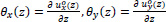
According to [16], if the displacements  of the point P are known, then the displacements us, un, uz of the random point M on the mean line of a thin-walled open cross-section, in the local coordinate system Μsnz (Fig. 2):
 |
(1) |
 |
(2) |
 |
(3) |
where:
are the degrees of freedom in the plane XOY O of the solid disk of the open section at the start point P.
us, un, uz are the displacements of point M along the local s, n and z-axis.
^α is the angle of the local s axis with the X 0 axis of the global coordinate system PX 0Y 0Z 0, which is a function of the dimension s.
Sm, Nm are the coordinates of point M in the global coordinate system PSNZ, which are functions of the dimension s.
 are the angles of the open cross-section about the horizontal axes x and y, respectively. These angles are functions of the dimension z.
 gives the change of the θz per unit length along Z-axis. This change is called twist and it constitutes the seventh degree of freedom, instead of the six known degrees of freedom of a common joint of a spatial structure.
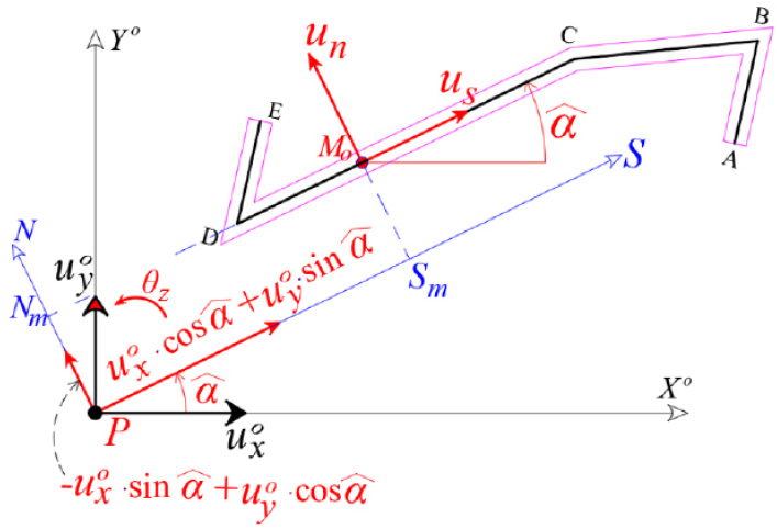
 is the function of the Sectorial Area or Sectorial Coordinate, of the point M («function of warping» or «measurement of warping»), Fig. (3). The parameter dω(s) is equal to the double area that is formed from the moving radius PM, where point M is shifted along the infinitesimal element on the mean line of the open section-leg. This area is considered positive when PM is rotated about Z-axis according to the rule of clockwised-screw (Cartesian System). The graphical display of the sectorial coordinate defines the distribution of the normal stresses on the open cross-section in the case of external bi-moment loading of the section, which is restrained against free torsion.
Eq. (3) yields that if a core with a thin-walled open cross-section is purely loaded with a torque about Z-axis, causing a unit twist of the section, i.e.
 |
then axial displacements are produced, which are numerically equal to the distribution of the sectorial coordinate ω(s):
 |
(4) |
By using the constitutive law of the material from the theory of elasticity, it is proved that the normal stresses acting on the cross-section are determined by:
 |
(5) |
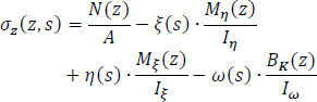
When the gravity principal directions ξ and η of the cross-section are rotated with respect to the gravity reference system Gxyz, Eq. (5) becomes:
 |
(6) |
where Iξ and Iη are the principal moments of inertia of the thin-walled open section about the principal axes ξ and η passing through the center of gravity G of the cross-section (local reference system Gξηz). The normal stresses resulting from the axial loading (1st term of Eq. 6) are superimposed and, also the normal stresses developed in the thin-walled open section due to bi-moment are superimposed (4th term of Eq. 6). It is noted that the positive sign in Eqs. (5-6) represents tensile stresses, while the negative sign represents compressive stresses on the cross-section. The sign of bending moments is taken positively when the moment vectors have the same sign with the positive semi-axis of the Cartesian reference system Gξηz.
In Eqs. (5-6), the meaning of the symbols is as follows:
ξ(s) and η(s) are functions of the cross-section coordinates in the local reference system Gξηz.
N(z) is the axial force (along the Z-axis) of the open section with area A and Modulus of Elasticity E:
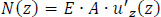 |
(7) |
Mx(z) and My(z) are the bending moments on the cross-section about the x and y-axis at the z level, according to Bernoulli's technical bending theory for prismatic beams. The quantity Iy represents the moment of inertia of the cross-section about the y-axis passing through the center of gravity G of the thin-walled open section, so that both the product second and first moments of area are zero:
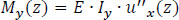 |
(8) |
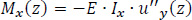 |
(9) |
Mξ(z) and Mη(z) are the bending moments acting on the thin-walled open section about the principal axes ξ and η, respectively, passing through the center of gravity G of the cross-section.
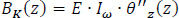
BK(z) is the bi-moment (or warping moment) at the z-level acting on the open cross-section.
Iω represents the warping or sectorial moment of inertia of the open cross-section with unit of length to the sixth power (m6). To calculate the torsional moment of inertia Iω, the following two conditions must always be met:
(i) Iω is calculated with respect to the Main Pole P of the cross-section, which coincides with the elastic center K (or stiffness center) of the thin-walled open cross-section and,
(ii) The principal start point MO(xO, yO) of the cross-section must always be used.
As long as these two cross-section conditions are satisfied, the torsional moment of inertia Iω becomes numerically minimal because both the product sectorial moments Ix,ω, Iy,ω (or Iξ,ω, Iη,ω depending on the reference system we are working in) as well as the sectorial first order moment of inertia Sω of the open cross-section become equal to zero:
 |
(10) |
where:
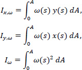 |
(11) |
To determine the location of the elastic center K (or center of stiffness) of the thin-walled open section, the following repeated procedure is proposed:
2.1. First Approximation
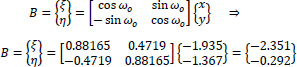
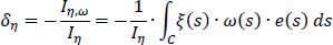
The goal to be achieved here is the product sectorial moments Iξ,ω and Iη,ω to be equal to zero. Having this goal, the equations for the calculation of the coordinates δξ and δη of the center of stiffness K(1) referring to pole P are:
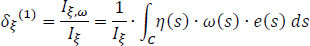 |
(12) |
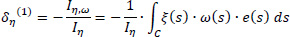 |
(13) |
where the exponent (1) shows the first approximation of the location of the elastic center K, ω(S) is the diagram of the sectorial areas of the cross-section referring to the temporary start point M, e(S) is the variable width of the core-leg as a function of the dimension s and ξ(S), η(S) are the known functions of coordinates in the local reference system Gξηz. During the first approximation, the product sectorial moments Iξ,ω and Iη,ω will not be zero (as they should be since they are calculated with reference to the real elastic center of the thin-walled open section), and therefore a second approximation is required.
Second Approximation: the point K(1) is considered now as the pole P while the same temporary start point M of the cross-section is used, and all calculations are repeated. The new corrected coordinates δξ(2) and δη(2) with respect to point K(1) are determined from Eqs. (12 and 13) and therefore, the corrected location of the elastic center is called K(2). If the deviation between the location of the elastic center of the cross-section into the last two approximations is not small and hence unaccepted, then we continue to a third approximation. To achieve convergence using this repeating procedure, the minimum number of required iterations is two or three, at least.
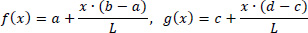
It is noted that since the functions x(s), y(s),η(S), ξ(S) and ω(S) present a linear variation along the straight legs of the mean line of the thin-walled open section, for the calculation of the above integrals some tabled formulas (integral of multiplication of two trapezoid diagrams) can be applied for each straight-line leg. For example, suppose that for a rectangular leg of length L and constant thickness e(x) = e, we have two linear, first degree, functions with respect to x, f(x) and g(x). Then for this special case, and to avoid analytical operations, the integral is given by the following relation:
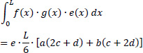 |
(14) |
where the symbols α, b, c and d are depicted in Fig. (4):
 |
In the case that the external action on a structural member is a torsional moment loading (either distributed or concentrated), the numerical calculation of the bi-moment diagram, or warping moment denoted by BK and measured in kN•m2, is done in a way completely analogous to the corresponding numerical calculation of the bending moment if instead of a loading of torsional moments we had a corresponding loading of forces (distributed or concentrated, respectively).
3. RESULTS AND DISCUSSION
3.1. Determination of the Principal Elastic System and of the Main Principle MO(xO, yO) of an open thin-walled section
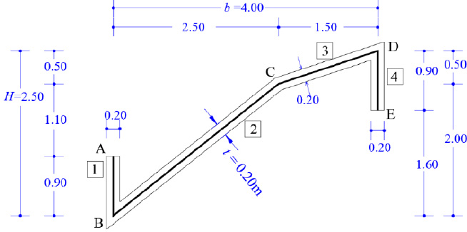
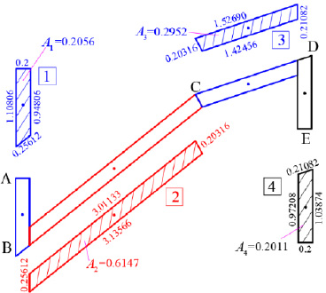
As a pilot numerical example, a thin-walled open cross-section will be examined in order to determine its principal reference system K(I,II,III) and the diagram of its sectorial coordinates through which the warping or sectorial moment of inertia Iω is finally calculated. The geometry of the thin-walled open section with constant width t = 0.20 m is shown in Fig. (5). It is noted that this asymmetric section can be found in folded plate structures. The cross-section in question has a thin-walled open form. Furthermore, we ideally divide the thin-walled open cross-section into four individual (not-rectangular) sections (1, 2, 3, 4), determine the center of gravity of each individual section (which is not analytically shown here, Fig. 6) and make the necessary calculations that are summarized in Table 1. Moreover, we can take an arbitrary temporary Cartesian 3D reference system OXYZ (Fig. 7) and geometrically draw the mean line of the thin-walled open cross-section. Next, we will calculate the center of gravity G as well as the principal directions ξ and η of the cross-section.
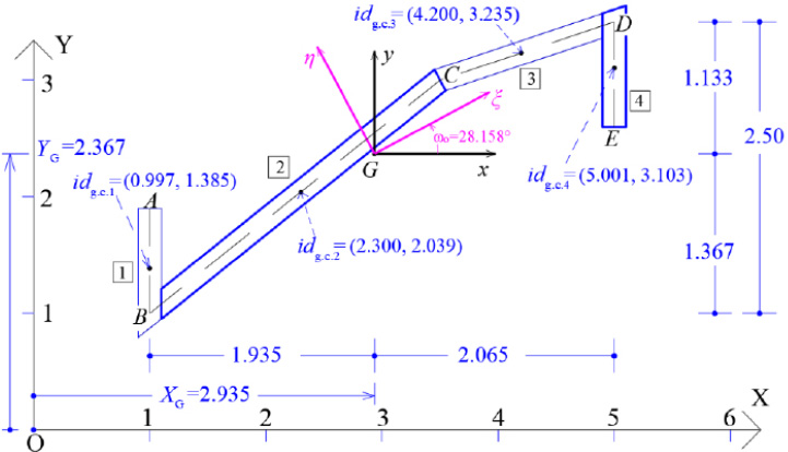
The coordinates (XG, YG) of the Center of Gravity G of the thin-walled open section with regard to the temporary reference system OXYZ, are:
 |
(15) |
 |
(16) |
We also consider the temporary Cartesian reference system Gxyz, (Fig. 7).
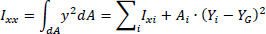
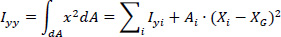
Then, we use Table 2 in order to calculate the moments of inertia of the open thin-walled cross-section relative to the Gxyz system. In the first two columns the coordinates x, y of the center of gravity of each individual leg i with respect to the center of gravity G of the cross-section are given. In column Ixi, the moment of inertia of each individual leg i with respect to the local axis parallel to x-axis, which passes through the center of gravity of the considered leg, is given. Correspondingly, in column Iyi, the moment of inertia of each individual leg i with respect to the local axis parallel to y-axis, that passes through the center of gravity of the considered leg, is given. Also, in column Ixyi, the moment of inertia of each individual leg i with respect to the local axes parallel to x and y axes, that pass through the center of gravity of the considered leg, is given. It is noted that the analytical calculations of these moments of inertia of each individual leg i are not shown here. In the next column Ixx, the moment of inertia of each leg i about the x-axis is calculated with respect to the center of gravity G of the cross-section (i.e. Ixi is increased according to the Steiner term, which is equal to the area Ai (Table 1) times the square of the distance to the x-axis, in other words Ai(Yi-YG)2. Similarly, in the next column Iyy, the moment of inertia of each leg i about the y-axis is calculated with respect to the center of gravity G of the cross-section (i.e. Iyi is increased by the Steiner term, which is equal to the area Ai times the square of the distance to the y-axis, Ai(Xi-XG)2. Finally, in the last column Ixy, the product moment of inertia is placed (i.e. Ixyi is increased by the Steiner term, which is equal for each leg i to the product of the area Ai with (Xi-XG)•(Yi-YG) .
The total moments of inertia of the thin-walled open section are given by:
 |
(17) |
 |
(18) |
 |
(19) |
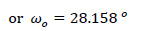
Additionally, we will calculate the orientation of the principal directions (ξ and η) of inertia of the thin-walled open cross-section determined by the angle ωO, regarding the Gxyz system:
 |
(20) |
 |
| Leg i | Xi-XG (m) of Center of Gravity of Leg | Yi-YG (m) of Centerof Gravity of Leg | Ix,i (m4) | Iy,i (m4) | Ιxy,i (m4) | Ixx (m4) | Iyy (m4) | Ixy (m4) |
|---|---|---|---|---|---|---|---|---|
| [1] | -1.938 | -0.983 | 0.01833 | 0.00068 | 0.00027 | 0.2168 | 0.7727 | 0.3917 |
| [2] | -0.635 | -0.328 | 0.19133 | 0.29530 | 0.23560 | 0.2576 | 0.5431 | 0.3637 |
| [3] | 1.265 | 0.867 | 0.00629 | 0.04832 | 0.01586 | 0.2281 | 0.5203 | 0.3395 |
| [4] | 2.066 | 0.735 | 0.01698 | 0.00067 | 0.00011 | 0.1257 | 0.8590 | 0.3056 |
| Sum | - | - | - | - | 0.25184 | 0.8282 | 2.6951 | 1.4005 |
Then, the principal moments of inertia (Iξ and Iη) of the thin-walled open cross-section about the principal axes ξ and η with origin the center of gravity G of the cross-section are calculated, as follows (Table 2):
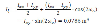 |
(21) |
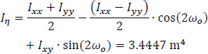 |
(22) |
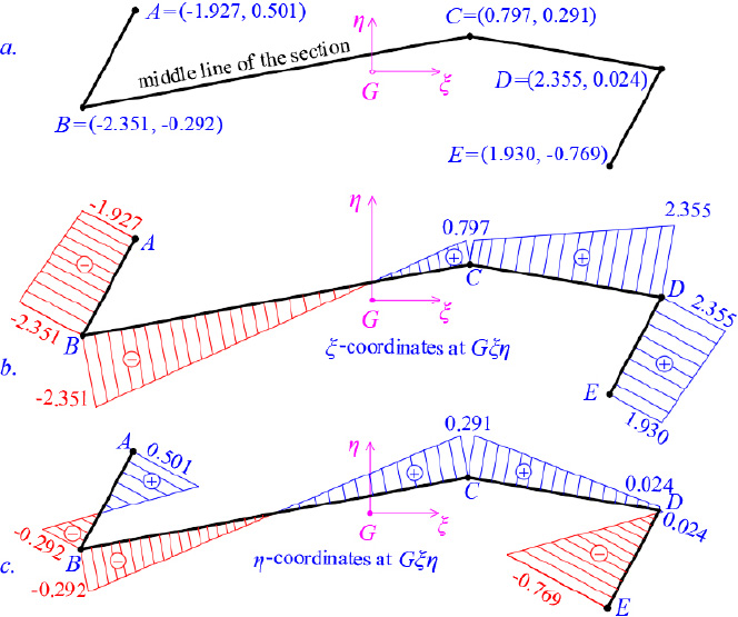
The coordinate diagrams ξ(s), η(s) of the thin-walled open cross-section at the Gξηz system are obtained either geometrically, or analytically using the rotation matrix:
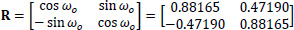 |
(23) |
As an example, point B has the following coordinates at the Gxyz system:

The coordinates of point B at the Gξηz system, which is rotated by  relative to the x-axis, are given below. Fig. (8) shows the coordinate diagrams ξ(s), η(s).
 |
(24) |
Next, the location of the elastic center K of the thin-walled open cross-section will be calculated. For this purpose, an iterative process is followed (usually at least two iterative steps are required to achieve convergence), which in the end always converges to the same point, which is the elastic center K of the open cross-section. The number of iterations depends on one hand on the choice of the arbitrary pole P that will be considered during the first approximation, and on the other hand on the position of the temporary start point M of the cross-section that is also chosen arbitrarily and remains fixed until the elastic center K is determined. Usually, to achieve a faster convergence of the iterative process in order to locate the elastic center K, we choose - in the first approximation the pole P to coincide with the geometric center G of the thin-walled open cross-section, while we must work at the Gξηz system.
3.2. Determination of the Elastic Center K(1) in 1st Approximation
The elastic center K of the cross-section presents an eccentricity with respect to the pole P (which coincides with the center of gravity G of the same cross-section at the first approximation). This eccentricity is determined by the coordinates δξ and δη with respect to G along the principal directions ξ and η, which are calculated from Εqs. (12 and 13), which are repeated below:
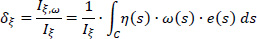 |
 |
where e(s) is the constant thickness of the section, ω(S)(1) is the diagram of the sectorial coordinates (sectorial area) of the cross-section with respect to the temporary start point M (Fig. 9), while ξ(s) and η(s) are known from the diagrams of Fig. (8). As regards the temporary start point M of the cross-section, it is recommended that some corner of the thin-walled cross-section can be chosen that is approximately in the middle of the mean line length of the cross-section, while the location of this start point M must be kept fixed for all the iterations to be performed. The location of the principal start point MO of the thin-walled open section will be calculated at the end, after finalizing the location of the elastic center K. In Tables 3 and 4, the calculations for finding the product warping moments Iη,ω and Iξ,ω are shown. The symbols a, b, c, d are used to apply Eq. (14). It is also emphasized here that the values of the two product warping moments (Iξ,ω, Iη,ω) are becoming zero when these are calculated with respect to the real elastic center K of the thin-walled open cross-section.
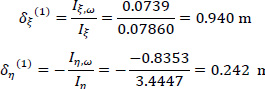
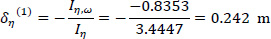
Therefore, using Eqs. (12 and 13) in a first approximation, the location of the elastic center K(1) with respect to the pole P (which here coincides with the center of gravity G) is (Fig. 9):
 |
 |

| ξ(s) | ω(s) | ||||||
|---|---|---|---|---|---|---|---|
| Leg | e (m) | Li (m) | a | b | c | d | Iη,ω (m5) |
| BA | 0.2 | 0.9 | -2.351 | -1.927 | 0 | -1.742 | 0.32427 |
| BC | 0.2 | 3.202 | -2.351 | 0.797 | 0 | -0.452 | 0.03652 |
| CD | 0.2 | 1.581 | 0.797 | 2.355 | -0.452 | -1.118 | -0.41853 |
| DE | 0.2 | 0.9 | 2.355 | 1.930 | -1.118 | -2.976 | -0.7776 |
| Sum | - | - | - | - | - | - | -0.8353 |
| η(s) | ω(s) | ||||||
|---|---|---|---|---|---|---|---|
| Leg | e | Li | a | b | c | d | Iξ,ω |
| BA | 0.2 | 0.9 | -0.292 | 0.501 | 0 | -1.742 | -0.0371 |
| BC | 0.2 | 3.202 | -0.292 | 0.291 | 0 | -0.452 | -0.0140 |
| CD | 0.2 | 1.581 | 0.291 | 0.024 | -0.452 | -1.118 | -0.0344 |
| DE | 0.2 | 0.9 | 0.024 | -0.769 | -1.118 | -2.047 | 0.1594 |
| Sum | - | - | - | - | - | - | 0.0739 |
3.3. DEtermination of the Elastic Center K(2) in 2nd Approximation
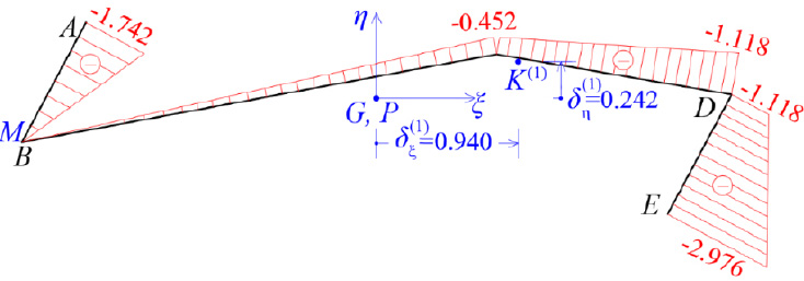
In the second approximation, the elastic center K(1) of the first approximation, which was calculated in the 1st approach, is used as the pole P, while the same temporary start point M of the cross-section (at point B) is used. In this second approximation, the sectorial diagram coordinates ω(S)(2) of the cross-section with respect to the temporary start point M, is given in Fig. (10). The calculations for finding the two product warping moments Iη,ω, Iξ,ω are shown in Tables 5 and 6.
| ξ(s) | ω(s) | ||||||
|---|---|---|---|---|---|---|---|
| Leg | e (m) | Li (m) | a | b | c | d | Iη,ω (m5) |
| BA | 0.2 | 0.9 | -2.351 | -1.927 | 0 | -2.384 | 0.4438 |
| BC | 0.2 | 3.202 | -2.351 | 0.797 | 0 | -0.238 | 0.0192 |
| CD | 0.2 | 1.581 | 0.797 | 2.355 | -0.238 | -0.276 | -0.1296 |
| DE | 0.2 | 0.9 | 2.355 | 1.930 | -0.276 | -1.492 | -0.3332 |
| Sum | - | - | - | - | - | - | 0.0002 |
| η(s) | ω(s) | ||||||
|---|---|---|---|---|---|---|---|
| Leg | e (m) | Li (m) | a | b | c | d | Iξ,ω (m5) |
| BA | 0.2 | 0.9 | -0.292 | 0.501 | 0 | -2.384 | -0.0508 |
| BC | 0.2 | 3.202 | -0.292 | 0.291 | 0 | -0.238 | -0.0074 |
| CD | 0.2 | 1.581 | 0.291 | 0.024 | -0.238 | -0.276 | -0.0125 |
| DE | 0.2 | 0.9 | 0.024 | -0.769 | -0.276 | -1.492 | 0.0737 |
| Sum | - | - | - | - | - | - | 0.0030 |
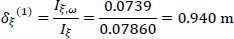
Therefore, using Eqs. (12 and 13) in a second approximation, the location of the elastic center K(2) with respect to the pole P (which here coincides with K(1)) is (Fig. 10):
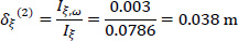 |
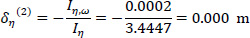 |
So, the corrected location of K from the center of gravity G is (Fig. 10):
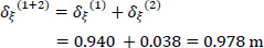 |
(25) |
 |
(26) |
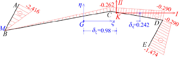
The accuracy achieved is very satisfactory and therefore no further approximation is required. However, if a third approximation is applied, then the final location of K is given as δξ(1+2+3) = 0.98m and δη(1+2+3) = 0.242m, and this position of the Elastic Center K is used in the following.
3.4. Calculation of the Corrected Sectorial Coordinate Diagram with Respect to the Final Location of the Elastic Center K
The final location of the elastic center K has been determined. Using pole K and with the same temporary start point M of the cross-section already obtained at point B, we correct the diagram of the sectorial coordinates ω(S)(M) of the cross-section (Fig. 11).
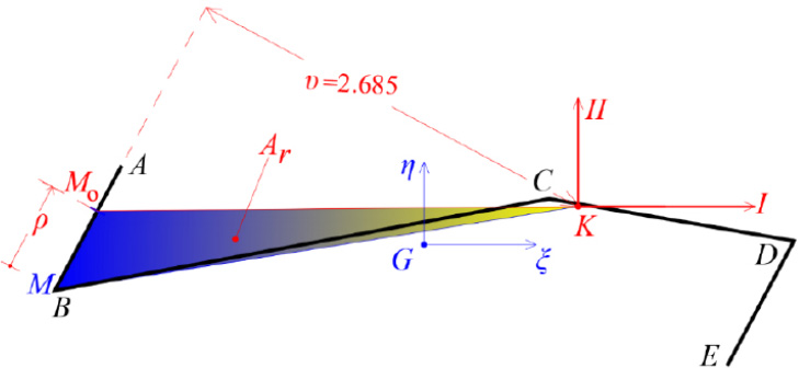
With the final location of the elastic center K known, and given the temporary start point M of the cross-section, we form the ideal triangle KMMo, with the point MO as unknown that must be determined. This is achieved by calculating the unknown distance ρ. The area Ar of the triangle KMMo is:
 |
(27) |
where υ is the height of the triangle which is known geometrically (Fig. 12).
Therefore, the distance ρ is given by:
 |
(28) |
| ω(s) | |||||
|---|---|---|---|---|---|
| Leg | e (m) | Li (m) | a | b |  |
| BA | 0.20 | 0.90 | 0 | -2.416 | -0.2174 |
| BC | 0.20 | 3.202 | 0 | -0.262 | -0.0839 |
| CD | 0.20 | 1.581 | -0.262 | -0.290 | -0.0873 |
| DE | 0.20 | 0.90 | -0.290 | -1.474 | -0.1588 |
| Sum | - | - | - | - | -0.5474 |
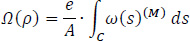
The magnitude 2Ar (i.e. twice the area of the triangle) represents the sectorial coordinate ω(s) of the triangle KMMo with the elastic center K as a pole and will be denoted by Ω(ρ) which is calculated from the following equation:
 |
(29) |
where A = 1.3165 m2 is the total area of the thin-walled cross-section (Τable 1), ω(S)(M) is the sectorial coordinates based on the temporary start point M and υ is the height of the triangle KMMo from K (Fig. 12), where υ is measured geometrically. The calculations for finding Ω(ρ) are shown in Table 7, in which the quantity is calculated.
If the quantity Ω(ρ) is negative, then the principal start point MO will be located with a negative rotation of the radius KM of the triangle KMMo (which is the case here).
Therefore, from Eq. (29):
 |
The height υ of the triangle KMMo is measured geometrically as 2.685 m, and consequently the distance ρ is calculated from Eq. (28):
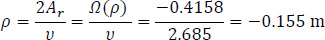 |
Being known the principal start point MO, the final corrected diagram of sectorial coordinates ω(s) is calculated, using the elastic center K as the pole (Fig. 13).
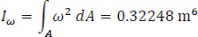
Then the value of the warping moment of inertia Iω of the thin-walled open cross-section is calculated, which will be used to calculate the positive normal stresses due to the external load of bi-moment BK for a specific level of the cross-section along the longitudinal dimension of the thin-walled structure.
The warping moment of inertia Iω (Eq. 11) of the thin-walled open section is calculated in Table 8 as:
 |
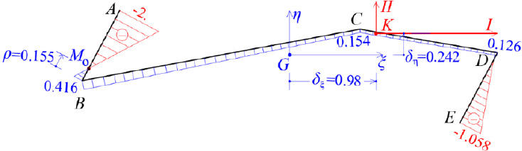
| ω(s) | ω(s) | ||||||
|---|---|---|---|---|---|---|---|
| Leg | e | Li | a | b | c | d | Iω |
| BA | 0.2 | 0.9 | 0.416 | -2. | 0.416 | -2. | 0.2008 |
| BC | 0.2 | 3.202 | 0.416 | 0.154 | 0.416 | 0.154 | 0.0557 |
| CD | 0.2 | 1.581 | 0.154 | 0.126 | 0.154 | 0.126 | 0.0062 |
| DE | 0.2 | 0.9 | 0.126 | -1.058 | 0.126 | -1.058 | 0.0601 |
| Sum | - | - | - | - | - | - | 0.32248 |
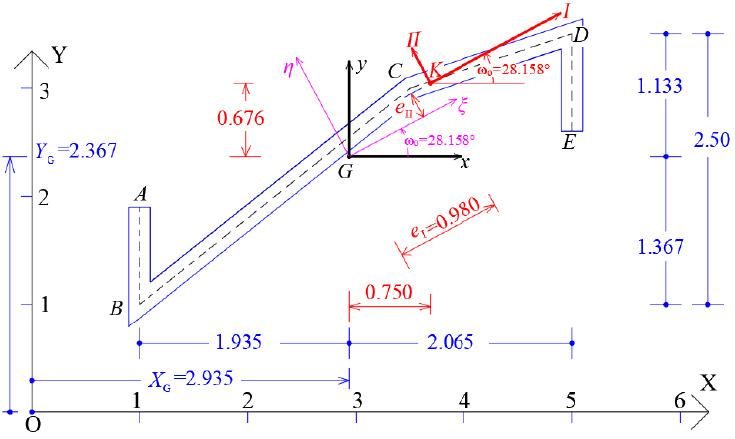
Fig. (14) shows the elastic principal system (K,I,II,III) of the thin-walled open cross-section with respect to the original reference system OXYZ, where the III-axis is the vertical axis passing through the elastic center K and together with the two horizontal axes I and II constitute the principal elastic reference system of the thin-walled open cross-section, with origin the elastic center K.
3.5. Calculation of Normal Stresses at the Middle Cross-section of the Folded Plate
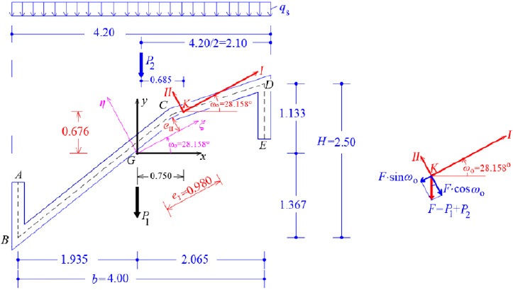
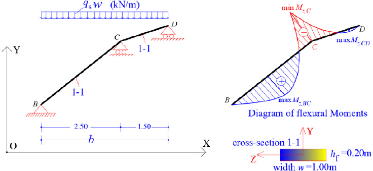
We consider the reinforced concrete (R/C) folded plate of Fig. (1), which has longitudinal dimension L = 20.00 m and is loaded with two loadings; (a) the self-weight (relative value 25 kN/m3) and (b) the projected-in-plan snow-weight qs = 4.00 kN/m2. Thus, the consultant forces of the two above-mentioned loadings are given (Fig. 15):
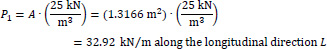 |
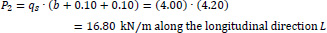 |
Next, the forces P1 and P2 are moving to Elastic Center K, hence, a torsional moment mt around the horizontal longitudinal axis III is the result:
mt = P1 x 0.75 + P2 x 0.685 = 32.92 x 0.75 + 16.80 x 0.685 = 36.20 kNm/m
’In addition, the consultant force F of P1 and P2 at the Elastic Center is:
F = P1 + P2 = 32.92 + 16.80 = 49.72 kN/m along the longitudinal direction L.
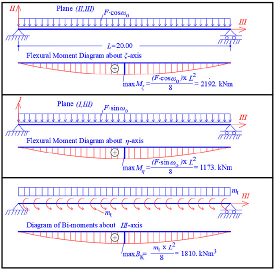
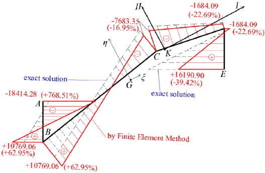
Furthermore, the force F is analyzed along the two Principal I and II-axes of the thin-walled open cross-section ABCDE (Fig. 15). Along the longitudinal direction, the folded plate is a prismatic beam (having thin-walled open cross-section) with hinges at both ends. Hence, there are two flexural moment diagrams at planes (II,III) and (I,III), as well as a bi-moment diagram due to torsional moment mt around the horizontal longitudinal axis III, as are shown in Fig. (16), where:
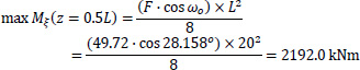 |
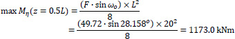 |
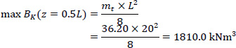 |
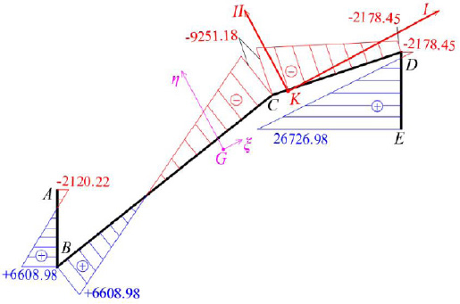
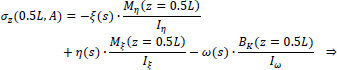
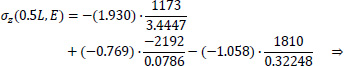
Therefore, the normal stresses σz(z,s) of the thin-walled open cross-section at the middle section of the longitudinal length of the folded plate, due to the simultaneous action of the forces P1 and P2 and their bi-moments, can be directly calculated from Eq. (6):
 |
In this equation, the first term is zero since there is not axial loading on the folded plate along the horizontal III-axis (i.e. N(z) = 0). All the necessary data to use the equation at the six points from A to E of the cross-section have already been calculated (ξ(S) and η(S) from Fig. (8), ω(S) from Fig. (13), Iξ = 0.0786m4, Iη = 3.4447m4 and Iω = 0.32248m6), while the normal σz(0.5L, S) diagram at the middle section of the folded plate with open thin-walled structure is as shown at Fig. (17). This is considered as the exact solution because all these come from the solving of closed mathematical relations derived from differential equations of the abovementioned “Bernoulli and Vlasov” theories.
Point A of the cross-section at the middle section of the folded plate along the longitudinal dimension (z = 0.5L):
 |
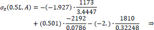 |
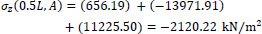 |
Point B of the cross-section at the middle section of the folded plate along the longitudinal dimension (z=0.5L):
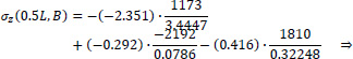 |
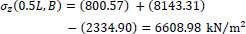 |
Point C of the cross-section at the middle section of the folded plate along the longitudinal dimension (z=0.5L):
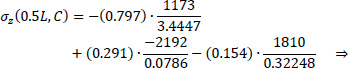 |
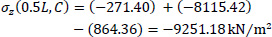 |
Point D of the cross-section at the middle section of the folded plate along the longitudinal dimension (z=0.5L):
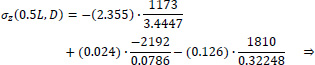 |
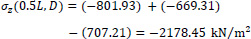 |
Point E of the cross-section at the middle section of the folded plate along the longitudinal dimension (z=0.5L):
 |
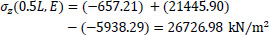 |
For comparison reasons, Fig. (18) shows the normal stress diagram σz(0.5L,s) derived from the F.E.M. analysis software SAP2000 [23] -using Modulus of Elasticity E = 30 GPa- with reference to the exact solution that comes from by the proposed present methodology. In the same Figure, we can see big differences where at point E is against safety (-39.42%).
It is worth noting that the analysis of the folded plate along the transverse dimension can be achieved as an inclined plate, with width w = 1.00 m, while we consider simple supports at the edges (at join of the folds) of the folded plate (Fig. 19).
CONCLUSION
In this paper, the exact determination of the principal elastic reference system of an RC folded plate having an asymmetric, thin-walled open section, and the calculation of the warping constant of this section, as well as the normal stresses (due to self-weight plus snow-weight) along the longitudinal dimension was presented. All calculations are carried out according to a recently modified technique [16] that examines the warping phenomenon of cores and is based on the Vlasov torsion theory [17, 18].
In the present article, the calculation of the warping properties of a thin-walled open cross-section is achieved by applying the following steps: (a) the location of the center of gravity G and the orientation of the principal axes ξ and η of the thin-walled open section are determined with respect to a temporary cartesian reference system OXYZ, (b) the principal moments of inertia Iξ and Iη of the thin-walled open section about the principal axes ξ passing through the gravity center G of the cross-section are calculated, (c) the diagrams of the coordinate-functions ξ(S) and η(S) of the thin-walled open section relative to the gravity reference system Gξηz are drawn, (d) the location of the elastic center K (stiffness center) of the thin-walled open section is calculated using a repetitive mathematical procedure, (e) the location of the principal start point MO(x 0, y 0) of the thin-walled open section is determined. It is worth noting that this start point is needed for the right calculation of the sectorial coordinates and for the calculation of the minimum numerical value of the warping moment of inertia Iω of the thin-walled open section, which is the exact value of Iω according to Vlasov torsion theory, (f) the numerical value of the warping moment of inertia Iω of the thin-walled open section is calculated, (g) the warping stiffness of the core is calculated and, last but not least, (h) the normal stresses at the middle section of a folded plate along the longitudinal dimension are calculated, considering the bi-axes flexure with the bi-moment phenomenon. All the above-mentioned properties give the exact solution of the folded plate in longitudinal dimension according to Bernoulli bending theory for prismatic beams (bending moments and axial force) and, additionally, according to Vlasov torsion theory (i.e. about the warping moment or bi-moment concept) for thin-walled open sections. This exact solution can be used for checking and assessment of the reliability of the results of various F.E.M. analysis software, since it is directly based on the superposition of Bernoulli bending theory and Vlasov torsion theory while the finite element method is approximate.
CONSENT FOR PUBLICATION
Not applicable.
AVAILABILITY OF DATA AND MATERIALS
Data and materials mentioned in the manuscript come solely from the authors. The data supporting the findings of the article is available within the article.
FUNDING
None.
CONFLICT OF INTEREST
The authors declare no conflict of interest, financial or otherwise.
ACKNOWLEDGEMENTS
Declared none.