All published articles of this journal are available on ScienceDirect.
Non-destructive Method of the Assessment of Stone Masonry by Artificial Neural Networks
Abstract
Background:
In this study , a methodology based on non-destructive tests was used to characterize historical masonry and later to obtain information regarding the mechanical parameters of these elements. Due to the historical and cultural value that these buildings represent, the maintenance and rehabilitation work are important to maintain the appreciation of history. The preservation of buildings classified as historical-cultural heritage is of social interest, since they are important to the history of society. Considering the research object as a historical building, it is not recommended to use destructive investigative techniques.
Objective:
This work contributes to the technical-scientific knowledge regarding the characterization of granite masonry based on geophysical, mechanical and neural networks techniques.
Methods:
The database was built using the GPR (Ground Penetrating Radar) method, sonic and dynamic tests, for the characterization of eight stone masonry walls constructed in a controlled environment. The mechanical characterization was performed with conventional tests of resistance to uniaxial compression, and the elastic modulus was the parameter used as output data of ANNs.
Results:
For the construction and selection of network architecture, some possible combinations of input data were defined, with variations in the number of hidden layer neurons (5, 10, 15, 20, 25 and 30 nodes), with 122 trained networks.
Conclusion:
A mechanical characterization tool was developed applying the Artificial Neural Networks (ANN), which may be used in historic granite walls. From all the trained ANNs, based on the errors attributed to the estimated elastic modulus, networks with acceptable errors were selected.
1. INTRODUCTION
The rehabilitation of historic buildings is considered an important step in the preservation of historical heritage, with a global or national dimension. For a well-grounded, lasting and with least possible damage rehabilitation process, non-destructive testing techniques (NDT’s) are available, which help in obtaining characteristics of the object to be analyzed. For this work, the following NDTs were used: the Ground Penetrating Radar (GPR) method, sonic tests and dynamic tests.
The GPR method consists basically in using a receiving antenna and an emitting antenna, which respectively, receive and emit electromagnetic waves to the subsurface and generate a characteristic radargram of the studied area [1]. Among the techniques of existing geophysical investigations, GPR (Ground Penetrating Radar) stands out for its efficient ability to generate images of the subsurface and the easy applicability to different situations. GPR was successfully used in investigations of historic buildings [2, 3]. The sonic tests are performed with an instrumented hammer and accelerometers for receiving waves, which can be P, R or S. The sonic tests are also widely used in the field of rehabilitation [4, 5]. Finally, there are dynamic tests, which provide the frequency and vibration modes of the analyzed structure. As the other methods presented, this one is also efficient in the characterization of structures [6, 7].
These techniques have been applied in masonry panels, built in a lab-controlled environment, with similar characteristics to existing historical buildings. Parallel to the application of NDTs, conventional uniaxial compression tests have also been carried out in the referred double-leaf granite stone masonry panels (DSM). These data were correlated with the results of NDTs with the aid of artificial neural networks (ANN); the elastic modulus was obtained by NDT’s.
The application of non-destructive tests on DSM, despite being an advanced technology, could be frustrating because the interpretation of the result is often difficult, as the masonry is a highly heterogeneous compound. The understanding of the mechanical behavior of masonry has been largely accomplished, due to the complexity of its nonlinear structural variables [8-12]. The combination of geophysical techniques in heritage buildings’ investigations ensures greater trust and complementary results.
The ambiguity inherent in the non-unicity of the response of the geophysical methods applied to masonry has led to the combined use of more than one of these methods to reduce the intrinsic uncertainty of the obtained models. The use of a synergy of NDTs, in parallel, in the same structure, as a support for the heritage preservation, brings many benefits to the analysis of the materials and the constructive elements. Through the analysis of specific parameters’ variations in each method, it is possible to obtain peculiar characteristics of the analyzed materials.
Artificial Neuronal Networks (ANN) are used as an option in this work since they are an efficient tool for correlating the results previously presented. ANNs are computational tools composed of interconnected processing units (artificial neurons) capable of solving complex problems in several areas of knowledge. They are based on the human neurological system behavior and therefore, can develop the ability to learn and store information, as well as recognize and classify patterns.
The networks have been successfully used in several works in the field of engineering [13-17]. ANNs in mechanical characterization analysis have also been used with success, as modeling compressive strength and failure criterion on the behavior of anisotropic materials such as masonry [18], could be used to predict the main cutting force component and the mean surface roughness during turning of tool steel [19], to predict the compressive strength of mortars [20, 21], the shear capacity of concrete beams [22] and the compressive strength of self-compacting concrete [23].
For each artificial neuron, several input data are defined, which may be original data or responses from other neurons in the network. All input data are received through a connection that has weight. Similarly, neurons also have a unique excitation threshold value, which is a minimum intensity for neuron activation. For a given response to exit one neuron and enter another, there must be an excitation threshold for the output and an activation function for the input. In this way, the synapse occurs depending on the weight signal and has an inhibitory (negative) or excitatory (positive) effect [24].
In general, the ANN trained with the use of a data set that is representative of the problem domain proves to be successful in solving new problems with reasonable accuracy. It is clear that while ANNs have been used successfully in numerous engineering applications, few studies have incorporated the use of them for the approach of the mechanical behavior of masonry [24-30].
The nntool (Neural Network Toolbox™) GUI (Graphical User Interface) neural network interface instrument, available in MatLab (Matrix Laboratory, 2013), was used to perform the data analysis since the same software contains a computational package for the use of ANN in its most diverse forms of processing. This package supports different types of networks, so it can be used for several areas of science and various types of problems.
For the construction of this ANN, the multi-layer feed-forward architecture was used as well as supervised learning with a backpropagation algorithm. The multilayer ANN was configured, trained and simulated using MatLab (Matrix Laboratory, 2013), through a code developed to automate this process.
The number of neurons in the input and output layer is defined by the problem. This setting is made empirically, but some selection criteria already presented in the literature are followed, namely: adopting a number of input neurons equal to the number of problem variables (which are set by the user); and starting with a hidden layer and with a number of neurons in that layer equal to the average input and output neurons.
After the definition of a set of samples to be analyzed, which corresponds to 70% of the samples, training data are randomly selected by the Matlab function (Matrix Laboratory, 2013) nntool for the neural network training. 15% of the samples are designated as validation data, which measure the generalization of the network, providing it with data that had not been seen before. The remaining 15% of the samples, called test data or simulation, provide an independent measure of neuronal network performance in terms of error rate. Through an iterative and random process, the weights are modified until the iterations converge to acceptable errors. In the training stage, the least possible mean square root error must be checked; the test set error and the validation set error must have similar characteristics and no significant overfitting should occur by iteration. With the weights already established, the network is subjected to validation and generalization through the sim function, responsible for the simulation through ANN. By following these checks, the best validation performance point is identified. After each training, the software reports the error graphs obtained for all samples, for each division. After the analysis of these graphs, the user requests, or not, new training of ANNs.
The performance of the network must be analyzed according to the relationship between the outputs and the corresponding targets. To improve the results, the following approaches can be used: restarting weights and re-training, increasing the number of hidden neurons, increasing the number of input data, and using another algorithm. In this work, the artificial neural networks were used to correlate the data of the NDT tests with the results of the mechanical tests. In this section, these variables used for the formation of the database of entry of ANNs are presented, as well as, the preparation of these data, obtained by the NDT tests, for later use in the ANN training.
For ANNs application, the user's role is to provide data that will be used in each step, i.e. sets of information (input and output) for training and validation and the input of generalization. Inputs are organized into arrays with their respective outputs and thus, the network recognizes the existing mathematical relationships between the data. In the present work, the input data set consists of samples corresponding to the results of the non-destructive tests organized in a column on an Excel sheet that is later imported into the workspace MatLab (Matrix Laboratory, 2013).
2. METHODOLOGY
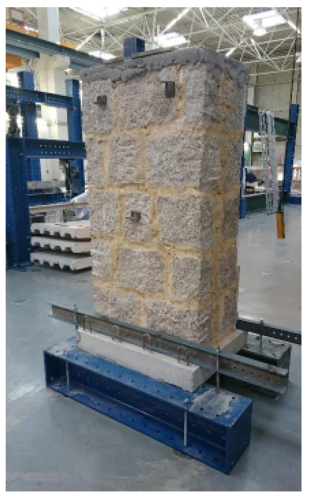
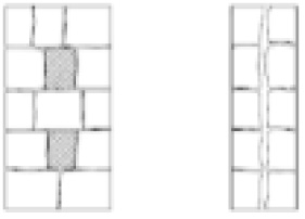
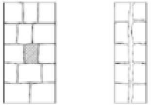
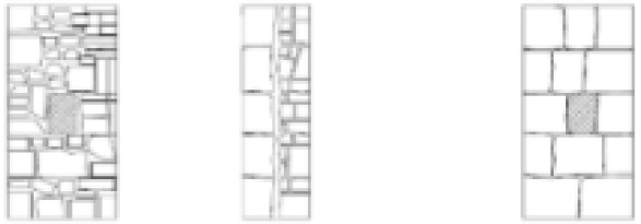
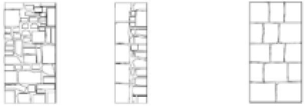
The investigations were carried out in the Laboratory of Seismic and Structural Engineering (LESE) of the Faculty of Engineering of the University of Porto (FEUP). Eight double-leaf stone masonry walls (DSM) were studied (Fig. 1) divided into four types (Table 1). The sequence of the work in the laboratory was performed in real scale masonry, using the parameters and techniques defined by the bibliography [31, 32].
| Characteristics | Layout (frontal / lateral) |
|---|---|
| Two-leaf regular (two cross block) PP1 and PP5 |
|
| Two-leaf regular (one cross block) PP2 and PP6 |
|
| Two-leaf regular and irregular (one cross block) PP3 and PP7 |
|
| Two-leaf regular and irregular (no cross block) PP4 and PP8 |
|
The eight DSM walls [32] are composed of a stone from the north of Portugal and a mortar consisting of hydrated lime, gravel, and water. The vertical and horizontal joints were considered approximately 3 cm thick. The masonry walls are made of granite blocks coarsely regulated, and a non-cohesive filler (small stone fragments bound with traditional lime mortar). The granite blocks used were collected from old masonry buildings located in the north of Portugal and mortars, composed of lime and clay (1:3 ratio). The masonry specimens were built by professionals under controlled laboratory conditions, idealized and constructed to be representative of the traditional typologies of masonry construction in the Mediterranean. The eight masonry walls are 0.90 m long, 0.55 m thick and 1.75 m high, leading to a slenderness rate h/t of 3.18 and a volume of 0.87 m3 each.
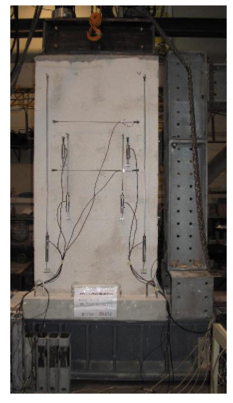
Table 2 presents an overview of the tests performed and the possible response variables used as input data for the neural networks. For the use of the GPR test (Fig. 2) as input data from the network, the variable chosen was the amplitude, represented by a value obtained after RMS (root-mean-square). The dynamic tests are represented by the values of the natural frequencies. The sonic tests will only be represented by the velocity values obtained with the indirect test configuration. The acronym VU represents unique values for the entire wall and VC represents specific values to each zone. Obtaining these values will be further detailed in the following subsection.
| NDT’s | Characteristics | Results |
|---|---|---|
| GPR (900 MHz) | amplitude | 3 x VC 1 |
| Dynamic | natural frequencies | VU 1 |
| Sonic (Indirect) | wave velocities | 3 x VC 2 |

It is important to note that the selected input data do not necessarily have to be correlated with each other, for example, the velocity values of the sonic wave propagation do not correlate with the values of the electromagnetic wave amplitudes. The purpose of ANN is to correlate these input parameters with the mechanical test data, namely the elastic modulus, so there is no need to correlate the input data with each other, but rather the existence of a correlation between the input data with the output data.
Information defined as input data should be standardized, since the discrepancy between the values of the information may result in the inadequate performance of the neural networks. For a correct training of the network, the database should cover as many possible scenarios of the structures, so that the network can handle the cases that may happen [17].
Table 3 presents an overview of the responses obtained with the uniaxial compression test that is used as ANN output data. The variable output is set to E2 (global tangent modulus panel - GPa -) resulting from compression testing. This variable was defined based on the slope of the graphs, compressive stress (σ) x Strains (ε), obtained by the results of the uniaxial compression tests (Fig. 3), for stress corresponding to the range of 20 to 40% of the maximum stress value (σmax) applied to each wall.
| Test | Characteristics | Result |
|---|---|---|
| Uniaxial compression test | E2 - Global tangent modulus panel | VU 2 |
The architecture of ANNs was defined based on six variables: geometric characteristics (presence of brakes and face characteristic - regular and irregular -), results of the dynamic characterization (vibration frequencies in the X and Y direction), wave velocity of indirect sonic tests (Ac1, Ac2 or Ac3) and the RMS values of the amplitudes of the GPR test. Thus, we considered one input layer with several neurons compatible with the number of input data, one hidden layer and one layer of output with one neuron. The network consists of 32 input samples (8 walls with 3 zones each, plus the average of each wall), with 192 data at the input base.
The data used must characterize the actual situation of the structure because they are strictly mathematical techniques so that the performance of the processing depends on the correct supply of data. Data normalization in the database (dynamic test results, sonic tests and GPR) is also advisable since the disparity between values can result in the detuned performance of the networks. This normalization was carried out by dividing all the values of each parameter by its identified maximum.
The number of neurons, which makes up the intermediate layers, was determined by a trial and error strategy. The network structure (number of layers and number of neurons) is associated with the adequate responsiveness of the trained network. To reduce the error obtained in the training phase, the number of neurons was increased until it became acceptable, without great variations. An initial attempt for the number of neurons in the intermediate layer was made according to Eq. (1):
 |
(1) |
Where: Nnci- number of neurons in the intermediate layer; Nvar,pe- number of variables in an input pattern; Natr- number of samples available for training.
In Eq. (2), Nvar,pe is number 6 because it represents the geometric characteristic (cross-block presence and irregular face presence); natural frequencies (x) and (y) from the dynamic tests; wave velocities from the indirect sonic tests (Ac3) and the amplitude from GPR. Natr is number 32, because the training was with 32 samples (eight DSM plus with the average for each of the three zones). The use of 5, 10, 15, 20, 25 and 30 neurons in the middle layer of the networks (Nnci) was tested.
 |
(2) |
The development and mathematical details of the implementation of ANNs can be seen in other reference works [33, 34], which are not debated here. The parameters used for the training of ANNs are summarized in Table 4.
| Parameter | Value |
|---|---|
| Training algorithm | Backpropagation algorithm |
| Number of hidden layers | 1 |
| Number of neurons per hidden layer | 5-30 by step 5 |
| Training goal | 0 |
| Epochs | 100 |
| Cost function | MSE (mean square error) |
| Transfer functions | Tansig |
After defining the ANN database, the next step is to perform training of the networks to achieve the most efficient tool. The efficiency of the trained network is defined in terms of the lowest error (%) calculated for each sample (Eq. 3).
 |
(3) |
Where: Target- are the values of E2; Output- the values provided by the training.
Network training consists of processing this data set (input and output) so that the tool can establish a mathematical relationship between them. Araújo (2017) suggests performing at least three runs with each test; in this way, the possibility of overfitting is reduced, and the convergence of the results is verified. The parameters that minimize the maximum relative error (Eq. 3) of the training data can be defined as follows:
- Data type analyzed: the larger the information in the input patterns, the more the algorithm establishes valid relations between input and output patterns;
- Network parameters (number of neurons): the number of neurons has a decisive role in network processing, since the higher the number, the better the performance. However, the exaggerated increase may lead to divergence of results.
2.1. Data Preparation for ANN’s
In this section, we present the methodology of organization of the database for six input variables of ANNs, as well as the adequacy of the responses of the NDTs to integrate into this base. It is worth mentioning that the responses of the dynamic characterization test did not suffer adequations, since their numerical values, which correspond to the vibration frequencies of the structure (1st and 2nd frequency), were thus included in the input database of ANN’s.
The input data were grouped in the matrix form. For the training and validation stages of networks with supervised learning, in the first phase, the input data are supplied together with their respective outputs, and, in this way, the network identifies the mathematical relationships between the information. In the second phase, the network parameters for training are defined, which include the type of algorithm, the number of neurons, the activation functions, the learning rate and the number of iterations. The algorithm tries to estimate the errors of this connection and, if acceptable, it proceeds to the validation phase, which is intended to evaluate the behavior of the trained network, using a set of unpublished data for the network (Araújo 2017).
It is important to emphasize that ANN is a tool developed to work with many samples in its database. This database is divided randomly as described above. In the last two phases (validation and testing), 15% of the data in the present study must correspond to a minimum of three samples, enough for the composition of an error chart. Therefore, a minimum set of 20 samples is required on this basis.
The number of samples (eight DSM) must be greater than the number of input variables; otherwise, this system will have more unknown data than equations for its resolution. Combination with only eight DSM walls is small to map the function implicit in this problem. To optimize the network result, there are two options: to reduce the size of the problem by decreasing the number of variables or to increase the number of samples.
Another issue is related to the difficulty in obtaining a large enough amount of experimental data capable of adequately training the ANN. It is obvious that producing too many samples is problematic and costly for sample production and actual measurement; during this period, it must be stored, and this requires specific space with the subsequent cost. An option was given to increase the number of samples, which should be at least triplicate. According to the configuration of the NDTs, three vertical zones were defined for characterization of each part of the DSM (Fig. 4).
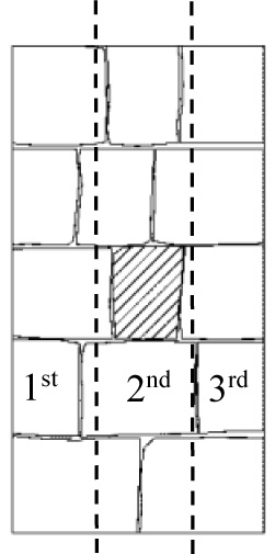
- 1st zone: alignment to the left of the cross-block.
- 2nd zone: cross-block alignment; and
- 3rd zone: alignment to the right of the cross-block.
The input data refers to the geometric characteristic (cross-block and irregular face) represented by a number. The DSM zone with no cross-block is represented as 0, one cross-block as 1 and two cross-block as 2, and also the irregular face presence is represented as 0 and its absence as 1.
The output data refer to the results of the uniaxial compression tests. According to the instrument used for the uniaxial compression test, we have LVDTs at both ends of each face. The first zone corresponds to the elastic modulus obtained by the graph referring to the mean of the LVDTs positioned in the left lateral zone (face A and B); the second zone corresponds to the elastic modulus obtained by the graph referring to the average of the 4 readings of the global LVDTs, since there is no instrumentation referring to this region during the test, and the 3rd zone corresponds to the mean of the LVDTs positioned in the right side zone (face A and B). The input variable for the dynamic test results is repeated 3 times, according to the characteristics of each vertical zone.
2.2. Sonic Tests Parameters
The results of the sonic tests, which were used as input data for the network, are those related to the indirect configuration. In fact, the tests with the direct configuration were not considered because they give results that characterize the walls punctually, and in the direction perpendicular to the application of the loads, reason why a good correlation with the module of deformability is not expected. It can be said that, for this type of masonry, the results of the direct sonic test, to some extent, depend on the compressive stress state in the masonry, but can be used to determine other characteristics of the masonry, such as the location of voids, joints and deterioration [35]. In this work, the results of the direct sonic tests were, however, important to frame and validate the results obtained by the indirect tests.
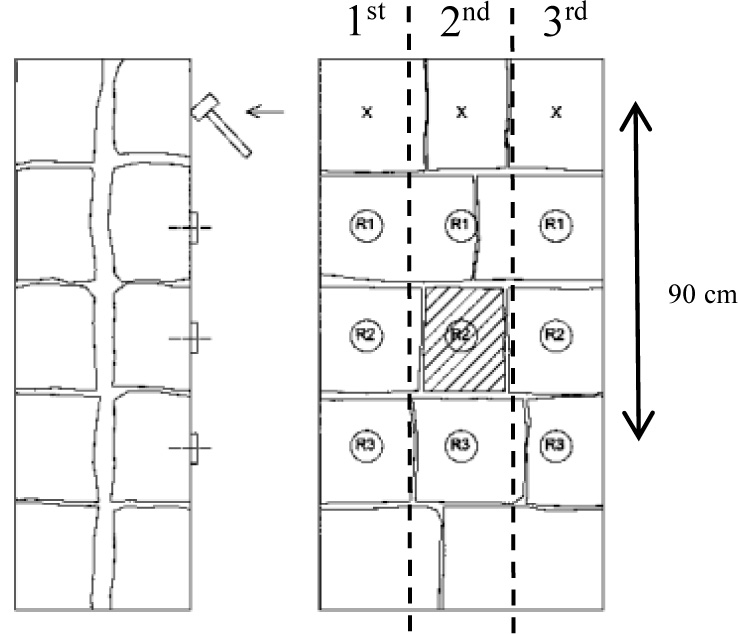
The accelerometer Ac3 (farthest) has, in the path made by the wave, 90 cm distance between the receiver and the emitter, thus involving an interaction with a major part of the wall structure. For this reason, its result was considered more characteristic. The accelerometer Ac2 is intermediate and Ac1 is the one with the shortest trajectory because it is closer to the emitter, involving less strains of masonry crossed by the wave, which is why the corresponding results are used here, but in a second sequence (Fig. 5).
2.3. GPR Tests Parameters.
The GPR test offers the radargrams as a response, from which data can be extracted related to the propagation velocity of the electromagnetic wave and the amplitude variations in the medium. This varies from point to point within the same radargram, so this characteristic was defined to numerically represent the results of this assay for ANNs. Based on the three zones defined for the walls (Fig. 4), the numerical data concerning the distribution of the amplitudes in the radargrams, referring to the XZ plane, according to Table 5, were exported.
The data of the radargrams chosen are exported as a numerical matrix, ie the values of the amplitudes vary according to the length and depth of each wall. These data are processed in MatLab software (Matrix Laboratory, 2013), with the RMS (root-mean-square) function. The processing sequence was as follows: first, an RMS is calculated for each column, and then an RMS is obtained with the values taken from all columns. This unique value, obtained at the end of the routine, is used to represent each zone of each wall as an input variable in the network.
To use the data resulting from the GPR tests as input data in the neural networks, it was necessary to define a methodology for converting radargrams into simple numerical data. In this way, these converted data represent the necessary variations between the samples for the ANN characterization. A characteristic behavior identified for each situation is thus obtained, so that a specific pattern can be verified. Table 6 presents the results obtained with the RMS for the amplitude data of each radar obtained, distributed according to typologies. The RMS values are related to the amplitude values of the radargrams, i.e., higher amplitudes are equivalent to higher RMS values.
 |
The amplitudes of the radargrams are influenced by the attenuations and reflections related to the medium crossed in the subsurface, thus, smaller amplitudes indicate bigger attenuations and smaller reflections. From the analysis of Table 6, we identified a variation pattern for the 2nd zone. The values of this zonewere for all the walls except for PP1, being smaller than the 1st and 3rd zone. As described, a lower RMS value indicates higher attenuations and smaller reflections. For this work, the smaller values of amplitudes can be attributed to smaller variations of the medium (fewer reflections), thus suggesting greater structural regularity. This is justified for walls PP5, PP2 and PP6 because in this second zone, there is an indication of the presence of the brakes, which offer greater structural stability to the walls.
The walls that have two leaves with the regular composition of the stones (PP1, PP2, PP5 and PP6) also present the lowest values of RMS, except for PP1. This may be related to the fact that they present greater structural stability than others, which have irregular leaflets (PP3, PP4, PP7 and PP8), also indicating greater regularity of the data.
2.4. Analysis Using Ann
In Table 7, the database used in the ANN analysis without normalization is shown. The six input parameters (geometric characteristics - cross-block presence and irregular face presence -; natural frequencies - x and y - from the dynamic tests; wave velocities from the indirect sonic tests - Ac3 - and the amplitude from GPR) and the output parameter (E2) are listed as previously described.
Varying combinations of DSM characteristics define the input patterns. Random combinations (R 1, R 2, R 3, R 4, R 5, R 6, R 7, R 8 and R 9) and six combinations according to the characteristics (RC, RCG, RCD, RES, RGPR and RCGF) were considered. As RC is a complete network, RCG is composed of the geometric characteristics (the presence and quantity of brakes in the masonry and the distinction between regular and irregular faces); RCD is composed of the dynamic characteristics; RCGF is composed of the characteristics obtained by the geophysical tests; RES is composed based on the results of the indirect sonic tests and RGPR is composed of the values of the amplitudes obtained by the GPR test. The activation function used between the layers, constant in the toolbox, was the Hyperbolic Tangent (Tansig) [18, 23, 21, 20]. The number of neurons in the hidden layer was also different (5, 10, 15, 20, 25 and 30 neurons). The characteristics of these networks are presented in Table 8.
Random combination networks are shown in Table 9, with net 3, 2 and 1 referring to the use of the input data of the Ac3, Ac2 and Ac1 accelerometer sonic tests, respectively. All networks were trained with a change in the number of neurons in the hidden layer (5, 10, 15, 20, 25 and 30), but the networks with end 2 and 1 referring to the use of the Ac2 and Ac1 sonic data, respectively, were trained with alterations of 15 and 30 neurons, which will be presented later. The number of the neurons for the networks with end 2 and 1 were selected after several trials.
The results of the training of the networks are presented below. It is worth mentioning that the training results of the networks with the presence of input data from the sonic tests, namely Ac2 and Ac1, are presented together at the end of the section. For the artificial neural networks for which the results are presented, the time required for calculation as a function of the number of selected neurons did not change significantly and is always less than one minute.
3. RESULTS OF ANN LEARNING
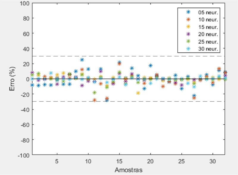
The RC3 (full network) training was performed in 32 samples; these data are comprised of the three zones plus the average of the three zones of each wall. After defining the number of samples, RC3 training was performed. The graph of Fig. (6) shows the error (%) obtained for each sample, in each training done with different numbers of neurons. Table 10 presents the training results in terms of the maximum relative error obtained (%) for each number of neurons used.
Although these error values are still significantly large (28%) for training, they are understandable. Given that the network must unveil an implicit behavior of a given phenomenon, if this phenomenon contains many variabilities, ANN will repeat this variability. That is, if there is a variability of up to 47% implied in the input data, then the network response with a 28% error is coherent. In addition, the RC3 network with 20 neurons reached a maximum error of 10%, which made its use feasible.
The results of the training of five networks with a combination of input data by types of tests (RCG, RCD, RCGF3, RES3 and RGPR), with variations in the number of neurons present in the hidden layer, are presented. The RCG is the network composed of the geometric characteristics, namely the presence and quantity of masonry brakes and the distinction between regular and irregular faces. The RCD is the network trained with input data regarding the dynamic characteristics, namely the natural frequency values in the directions x and y. RCGF3 is the network trained with input data referring to the characteristics obtained with the geophysical tests (GPR and indirect sonic tests of Ac3), specifically the average value of the amplitude and the speed of propagation of the wave. RES3 is the network trained only with input data concerning the results of the indirect sonic assays of the Ac3, i.e., the wave propagation velocity. RGPR is the network trained only with input data referring to the values of the amplitudes obtained by the GPR test.
These trained networks RCG, RCD, RES3, RGPR and RCGF3, present high error values for all numbers of neurons, 5, 10, 15, 20, 25 and 30. After analyzing the relative error results of these, in the case of the trained networks, presented in Table 11, it is concluded that the use of this simulation tool, with this distribution of input data, is not feasible since the error rates reached are high, all above 30%. Except for RCD networks for 5, 20, 25 and 30 neurons, RGPR for 25 neurons and RCGF3 for 30 neuronspresented errors less than or equal to 30%. The networks considered viable are highlighted in green in this table.
| Amplitude (dB) | ||||||||
|---|---|---|---|---|---|---|---|---|
| DSM | PP1 | PP5 | PP2 | PP6 | PP3 | PP7 | PP4 | PP8 |
| 1st zone | 7.43E+03 | 6.02E+03 | 6.21E+03 | 5.86E+03 | 8.16E+03 | 9.40E+03 | 7.88E+03 | 8.65E+03 |
| 2nd zone | 7.00E+03 | 3.82E+03 | 5.36E+03 | 4.55E+03 | 6.80E+03 | 6.70E+03 | 6.31E+03 | 6.35E+03 |
| 3rd zone | 5.86E+03 | 6.97E+03 | 6.69E+03 | 5.01E+03 | 8.31E+03 | 7.94E+03 | 7.31E+03 | 8.12E+03 |
| DSM | Zone | Cross-Block | Irreg. Face | Freq. x (Hz) | Freq. Y (Hz) | Vel. Ac3 (m/s) | GPR Amp. (dB) | E2 (Gpa) |
|---|---|---|---|---|---|---|---|---|
| PP1 | 1st | 0 | 1 | 13.30 | 10.10 | 421.00 | 7431.26 | 0.18 |
| 2nd | 2 | 1 | 13.30 | 10.10 | 484.00 | 6998.95 | 0.18 | |
| 3rd | 0 | 1 | 13.30 | 10.10 | 437.00 | 5858.85 | 0.20 | |
| Avg. | 2 | 1 | 13.30 | 10.10 | 447.33 | 6763.02 | 0.19 | |
| PP2 | 1st | 0 | 1 | 11.60 | 9.80 | 1023.00 | 6208.61 | 0.19 |
| 2nd | 1 | 1 | 11.60 | 9.80 | 1184.00 | 5363.31 | 0.17 | |
| 3rd | 0 | 1 | 11.60 | 9.80 | 938.00 | 6687.11 | 0.16 | |
| Avg. | 1 | 1 | 11.60 | 9.80 | 1048.33 | 6086.34 | 0.17 | |
| PP3 | 1st | 0 | 0 | 13.10 | 9.50 | 511.00 | 8164.74 | 0.16 |
| 2nd | 1 | 0 | 13.10 | 9.50 | 662.00 | 6796.37 | 0.13 | |
| 3rd | 0 | 0 | 13.10 | 9.50 | 363.00 | 8312.87 | 0.10 | |
| Avg. | 1 | 0 | 13.10 | 9.50 | 512.00 | 7757.99 | 0.13 | |
| PP4 | 1st | 0 | 0 | 12.30 | 6.90 | 634.00 | 7875.86 | 0.12 |
| 2nd | 0 | 0 | 12.30 | 6.90 | 523.00 | 6310.56 | 0.14 | |
| 3rd | 0 | 0 | 12.30 | 6.90 | 634.00 | 7306.82 | 0.19 | |
| Avg. | 0 | 0 | 12.30 | 6.90 | 597.00 | 7164.41 | 0.15 | |
| PP5 | 1st | 0 | 1 | 12.60 | 10.20 | 865.00 | 6017.91 | 0.31 |
| 2nd | 2 | 1 | 12.60 | 10.20 | 464.00 | 3815.68 | 0.24 | |
| 3rd | 0 | 1 | 12.60 | 10.20 | 592.00 | 6972.63 | 0.19 | |
| Avg. | 2 | 1 | 12.60 | 10.20 | 640.33 | 5602.08 | 0.25 | |
| PP6 | 1st | 0 | 1 | 18.00 | 9.00 | 1500.00 | 5860.59 | 0.30 |
| 2nd | 1 | 1 | 18.00 | 9.00 | 1731.00 | 4549.62 | 0.27 | |
| 3rd | 0 | 1 | 18.00 | 9.00 | 1071.00 | 5005.30 | 0.26 | |
| Avg. | 1 | 1 | 18.00 | 9.00 | 1434.00 | 5138.50 | 0.28 | |
| PP7 | 1st | 0 | 0 | 14.70 | 7.70 | 1250.00 | 9397.70 | 0.14 |
| 2nd | 1 | 0 | 14.70 | 7.70 | 1154.00 | 6700.97 | 0.13 | |
| 3rd | 0 | 0 | 14.70 | 7.70 | 1184.00 | 7937.21 | 0.12 | |
| Avg. | 1 | 0 | 14.70 | 7.70 | 1196.00 | 8011.96 | 0.13 | |
| PP8 | 1st | 0 | 0 | 14.60 | 7.40 | 1731.00 | 8649.52 | 0.22 |
| 2nd | 0 | 0 | 14.60 | 7.40 | 1667.00 | 6352.85 | 0.19 | |
| 3rd | 0 | 0 | 14.60 | 7.40 | 1216.00 | 8118.00 | 0.17 | |
| Avg. | 0 | 0 | 14.60 | 7.40 | 1538.00 | 7706.79 | 0.19 |
| ANN | Input | Number of Neurons | Output |
|---|---|---|---|
| RC3 | Cross-block presence; Irregular face presence; frequency (x); frequency (y); Sonic Indirect Ac3; Amplitude GPR | 5, 10, 15, 20, 25, 30 | E2 (GPa) |
| RC2 | Cross-block presence; Irregular face presence; frequency (x); frequency (y); Sonic Indirect Ac2; Amplitude GPR | 15, 30 | |
| RC1 | Cross-block presence; Irregular face presence; frequency (x); frequency (y); Sonic Indirect Ac1; Amplitude GPR | ||
| RCG | Cross-block presence; Irregular face presence; |
5, 10, 15, 20, 25, 30 | |
| RCD | frequency (x); frequency (y); | ||
| RCGF3 | Sonic Indirect Ac3; Amplitude GPR | ||
| RCGF2 | Sonic Indirect Ac2; Amplitude GPR | 15, 30 | |
| RCGF1 | Sonic Indirect Ac1; Amplitude GPR | ||
| RES3 | Sonic Indirect Ac3; | 5, 10, 15, 20, 25, 30 | |
| RES2 | Sonic Indirect Ac2; | 15, 30 | |
| RES1 | Sonic Indirect Ac1; | ||
| RGPR | Amplitude GPR | 5, 10, 15, 20, 25, 30 |
| ANN | Regular/irreg. Leaf | Cross-block Presence | Dyn. X | Dyn. Y | Sonic Ac3 | Sonic Ac2 | Sonic Ac1 | GPR Amp. |
|---|---|---|---|---|---|---|---|---|
| R1-3 | X | X | X | X | ||||
| R1-2 | X | X | X | X | ||||
| R1-1 | X | X | X | X | ||||
| R2-3 | X | X | X | |||||
| R2-2 | X | X | X | |||||
| R2-1 | X | X | X | |||||
| R3 | X | X | X | |||||
| R4 | X | X | X | X | ||||
| R5-3 | X | X | X | X | X | |||
| R5-2 | X | X | X | X | X | |||
| R5-1 | X | X | X | X | X | |||
| R6 | X | X | X | X | X | |||
| R7-3 | X | X | X | |||||
| R7-2 | X | X | X | |||||
| R7-1 | X | X | X | |||||
| R8 | X | X | X | |||||
| R9-3 | X | X | X | X | ||||
| R9-2 | X | X | X | X | ||||
| R9-1 | X | X | X | X |
| Number of Neurons | Relative Error Max. Absolute (%) |
|---|---|
| 05 | |-28| |
| 10 | |-28| |
| 15 | |-19| |
| 20 | |10| |
| 25 | |-18| |
| 30 | |-11| |
| Number of Neurons | Maximum Relative Error Approx. (%) | ||||
|---|---|---|---|---|---|
| RCG | RCD | RES3 | RGPR | RCGF3 | |
| 05 | -54 | -27 | -52 | -60 | -38 |
| 10 | -65 | -31 | -41 | -42 | -33 |
| 15 | -58 | -31 | -57 | -36 | 35 |
| 20 | -59 | -30 | -45 | -62 | -41 |
| 25 | -54 | -30 | -38 | -26 | 31 |
| 30 | -65 | -30 | -54 | -35 | -25 |

The following are the training results of the nine randomly combined networks (R1-3, R2-3, R3, R4, R5-3, R6, R7-3, R8 and R9-3), with variations in the number of neurons present in the hidden bed. R1-3 is the trained network with input data based on the results obtained with GPR, sonic (Ac3) and geometric characteristics. R2-3 is the trained network with input data based on the results obtained with the indirect sonic tests (Ac3) and the geometric characteristics. R3 is the trained network with input data based on the results obtained with the GPR (mean amplitude values) and geometric characteristics. R4 is the trained network with input data related to the results obtained with dynamic tests (natural frequencies x and y) and geometric characteristics. R5-3 is the trained network with input data referring to the results obtained with dynamic tests (natural frequencies x and y), geometric characteristics and indirect sonics (Ac3). R6 is the trained network with input data related to the results obtained with the dynamic tests (natural frequencies x and y), geometric characteristics and the GPR (mean amplitude) tests. R7-3 is the trained network with input data based on the results obtained with dynamic and sonic tests (Ac3). R8 is the trained network with input data based on the results obtained with the dynamic tests and the GPR. R9-3 is the trained network with input data referring to the results obtained with dynamic tests, GPR and sonic (Ac3) (Fig. 7).
These trained networks R1-3, R2-3, R3, R4, R5-3, R6, R7-3, R8 and R9-3 have error values with large variations between -67% and - 8%, for all numbers of neurons, 5, 10, 15, 20, 25 and 30. Among them, networks with higher errors (above 30%) are not considered for use. The R1-3 network is not indicated with 20 and 25 neurons. For the R2-3 network, only its use with 30 neurons is indicated. The R3 network is not indicated with any number of neurons. The R4 network is indicated with only 20 neurons. The R5-3 network is not indicated only with five neurons. The R6 network is indicated with 20 and 30 neurons. The R7-3 network is not indicated only with 10 neurons. The R8 network is indicated only with 10 and 30 neurons, and the R9 network is indicated for all numbers of trained neurons. The indicated networks are highlighted in green in Table 12.
After analyzing the relative error results of the trained networks presented in Table 12, it is concluded that the use of the R9-3 tool, with this input data distribution, is feasible and efficient since the error rate reached was -8%, with the use of 30 neurons.
After training of the 90 nets mentioned above, analyses were performed on the results obtained to verify which trainings obtained the highest efficiency in relation to the number of neurons, considering the error rates. The lowest error rates were obtained with architectures with 30, 20 and 15 neurons in the hidden layer of the networks. For this new training phase, with accelerometer changes (Ac1 and Ac2) in the sonic tests, 16 types of networks were defined and trained: RC1, RC2, RCGF1, RCGF2, RES1, RES2, R1-1, R1 -2, R2-1, R2-2, R5-1, R5-2, R7-1, R7-2, R9-1 and R9-2. After analyzing the behavior against the number of neurons only for networks with sonic test inputs, the best results with respect to the error rates were obtained with 15 and 30 neurons. Therefore, the following procedures were followed for variants of 15 and 30 in the number of neurons.
According to the orientation described previously, the networks R1, R2 and RES, using results of Ac1 and Ac2, obtained unsatisfactory results. These networks have in common the absence of dynamic results as input data from the network. The most efficient networks are R9-1, R7-1 and R5-1 with 30 neurons and RC2 with 15 neurons. These have in common the presence of dynamic and sonic results as input data.
Table 13 presents the results that present the networks with more efficient simulation, with eras referring to values of E2 (GPa) of less than 20%. These simulation tools can be applied more safely in the final response.
The 44 networks that presented error rates between 20% and 30% (Table 14) were considered possible tools to use, but in a secondary way. The other networks, with error rates up to 30%, were not used and were removed .
| Number of Neurons | Maximum Relative Error. (%) | ||||||||
|---|---|---|---|---|---|---|---|---|---|
| R1-3 | R2-3 | R3 | R4 | R5-3 | R6 | R7-3 | R8 | R9-3 | |
| 05 | -30 | -50 | -58 | -42 | -46 | -45 | -30 | -38 | 22 |
| 10 | -27 | -47 | -54 | -33 | 24 | -32 | -34 | 24 | 20 |
| 15 | 24 | -37 | -55 | -32 | -29 | -53 | -30 | 37 | -13 |
| 20 | -35 | -67 | 38 | -29 | -25 | -29 | 26 | -56 | -19 |
| 25 | -43 | -42 | -61 | 38 | -28 | -53 | -25 | -33 | -13 |
| 30 | -27 | 30 | -51 | -33 | -30 | -22 | -29 | 23 | -8 |
| ANN | Absolute Maximum Relative Error (%) | ANN | Absolute Maximum Relative Error (%) |
|---|---|---|---|
| R9.30.Ac3 | |-8| | R9.30.Ac1 | |-16| |
| RC.20.Ac3 | |10| | RC.25.Ac3 | |-18| |
| RC.30.Ac3 | |-11| | R9.20.Ac3 | |-19| |
| R9.15.Ac1 | |-13| | RC.15.Ac2 | |19| |
| R9.15.Ac3 | |-13| | RC.15.Ac3 | |-19| |
| R9.25.Ac3 | |-13| | R5.30.Ac1 | |-20| |
| R7.30.Ac1 | |16| | R9.10.Ac3 | |20| |
| ANN | Absolute Maximum Relative Error (%) | ANN | Absolute Maximum Relative Error (%) |
|---|---|---|---|
| R6.30 | |-22| | R5.25.Ac3 | |-28| |
| R7.15.Ac1 | |22| | R7.15.Ac2 | |-28| |
| R9.05.Ac3 | |22| | RC.05.Ac3 | |-28| |
| R8.30 | |23| | RC.10.Ac3 | |-28| |
| R1.15.Ac3 | |24| | RC.30.Ac1 | |28| |
| R5.10.Ac3 | |24| | R1.30.Ac2 | |-29| |
| R5.15.Ac1 | |-24| | R4.20 | |-29| |
| R8.10 | |24| | R5.15.Ac3 | |-29| |
| RC.30.Ac2 | |-24| | R6.20 | |-29| |
| R5.20.Ac3 | |-25| | R7.30.Ac3 | |-29| |
| R7.25.Ac3 | |-25| | RCGF.15.Ac1 | |29| |
| RCGF.30.Ac3 | |-25| | R1.05.Ac3 | |-30| |
| R7.20.Ac3 | |26| | R2.30.Ac3 | |30| |
| R9.15.Ac2 | |26| | R5.15.Ac2 | |-30| |
| R9.30.Ac2 | |-26| | R5.30.Ac3 | |-30| |
| RGPR.25 | |-26| | R7.05.Ac3 | |-30| |
| R1.10.Ac3 | |-27| | R7.15.Ac3 | |-30| |
| R1.30.Ac3 | |-27| | RCD.20 | |-30| |
| R5.30.Ac2 | |-27| | RCD.25 | |-30| |
| RC.15.Ac1 | |27| | RCD.30 | |-30| |
| RCD.05 | |-27| | RCGF.30.Ac1 | |-30| |
| RCGF.15.Ac2 | |-27| | RCGF.30.Ac2 | |30| |
Although these error values are high (30%), they are understandable. The network must translate an implicit behavior of a given phenomenon, if this phenomenon contains many variabilities, the ANN will repeat this variability. That is, there is a variability of up to 47% implicit in the input data, so the network response with 30% error is coherent. In addition, R9.30.Ac3 network with 30 neurons reached a maximum error of 8%, which made its use feasible.
CONCLUSION
The networks were used to develop a simulation tool capable of mechanically characterizing (namely elastic modulus) the double-walled granite wall samples with some variations, such as the presence of brakes and the regularity of the faces. In addition, variations in input data and network architecture (number of neurons) were tested, with 122 networks trained.
With the analysis of the training performed, it was concluded that only 10% of the trained networks (without variation 1 and 2, corresponding to Ac1 and Ac2 respectively) presented satisfactory results, that is, (<20%), namely R9-3 (with 10, 15, 20, 25 and 30 neurons) and RC3 (with 15, 20, 25 and 30 neurons). These networks considered to be “optimal” were obtained with the use of all the tests as input data. However, the trained networks with only one input variable presented the highest error values (RCG, RGPR, RES and RCD). This corroborates the idea that the synergy of the tests used was essential to efficiently translate the characteristics of the granite masonry samples into these networks.
It was also possible to conclude that the increase in the number of neurons present in the hidden layer leads to a better performance of the network since all trained networks with only five neurons obtained unsatisfactory results. Moreover, for the networks trained with the Ac2 accelerometer variant (sonic tests), only the RC2 network (with 15 neurons) that obtained an error of less than 20%, can then also be used as a simulation tool to characterize these structures. On the other hand, the networks trained with the Ac1 accelerometer variation (sonic tests)also obtained error values lower than 20%, which were R5-1, R7-1 and R9-1, for which data was obtained by sonic and dynamic tests. This highlights the importance of using these types of nondestructive tests to characterize the study material.
After performing this series of ANN training, it was possible to verify that the variables defined as input data to numerically represent the results of each NDT test, ie, the velocity of the sonic wave as a response of the indirect sonic tests (Ac1, Ac2 and Ac3), the RMS of the radargrams amplitudes obtained by the GPR test, the natural vibration frequencies (1st and 2nd frequency) in response to the dynamic characterization tests, were convincing because they achieved relevant results. The simulation tools obtained in this work can be used for several case studies, since these present similar characteristics to the samples that compose this database.
This study might help in overcoming costly and time-consuming experiments. The proposed tool is better than mechanically characterizing masonry panels with conventional mechanical tests, because in the case of historical masonry, their structural preservation is essential in the maintenance and rehabilitation work of the historical buildings. Conventional mechanical tests damage structures, and this problem has been eradicated by using ANN with the aid of NDTs, being the novel contribution of the study.
The main advantage of a trained ANN over conventional numerical analysis procedures is that the results can be produced with much less computational effort. The use of ANNs can assist decisively in the design of a restoration masonry, minimizing time and resources. However, it is important to highlight that the extension of the database used in this project with more DSM entries will further increase accuracy.
These tools were applied in some case studies that showed efficient use of this simulation, as it exhibited a deviation of less than 5%, since the ANN input data have been obtained correctly. This confirms the feasibility of using these simulation tools to assist the characterization processes of traditional and historical buildings with granite stone masonry.
CONSENT FOR PUBLICATION
Not applicable.
AVAILABILITY OF DATA AND MATERIALS
The data supporting the findings of the article is available in the Repositório Aberto da Universidade do Porto at https://repositorio-aberto.up.pt/handle/10216/122308, reference number 101542623.
FUNDING
The authors would like to thank CEFET-MG (CentroFederal de Educação Tecnológica de Minas Gerais-Brasil)and CAPES - Coordenação de Aperfeiçoamento de Pessoal deNível Superior/Brasil - for financial support (Process number0841/14-5). Also, this work was financially supported by:Project POCI-01-0145-FEDER-007457-CONSTRUCT-Institute of R&D In Structures and Construction funded by FEDER funds through COMPETE2020-Programa Operacional Competitividade e Internacionalização (POCI) -and by national funds through FCT - Fundação para a Ciência ea Tecnologia.
CONFLICT OF INTEREST
The author declares no conflict of interest, financial or otherwise.
ACKNOWLEDGEMENTS
The authors thank the technicians of the Laboratory for Earthquake and Structural Engineering (LESE) of FEUP, for their assistance with the experimental tests.

