All published articles of this journal are available on ScienceDirect.

Seismic Assessment of Steel MRFs by Cyclic Pushover Analysis
Abstract
Background:
Structural members subjected to strong earthquakes undergo stiffness and strength degradation. To predict accurately the seismic behaviour of structures, nonlinear static methods of analysis have been developed in scientific literature. Generally, nonlinear static methods perform the pushover analysis by applying a monotonic lateral load. However, every earthquake input is characterized by several repeated loads with reverse in signs and the strength and deformation capacities of structures are generally related to the cumulative damage. This aspect is neglected by the conventional monotonic approaches, which tend to overestimate the strength and stiffness of structural members.
Objective:
This paper aims to investigate the possibility that the Cyclic Pushover Analysis (CPA) may be used as a tool to assess the seismic behaviour of structures. During the CPA, the structure is subjected to a distribution of horizontal forces that is reversed in sign when predefined peak displacements of the reference node are attained. This process repeats in cycles previously determined in a loading protocol.
Methods:
To investigate the effectiveness of the CPA in predicting the structural response, a steel moment resisting frame is designed as a case study building. A numerical model of this frame is developed in OpenSees. To examine the influence of the loading protocols on the seismic response, the CPA is run following the ATC-24 and the SAC protocols. Additionally, the seismic demand of the case study frame is determined by a Monotonic Pushover Analysis (MPA) and by Incremental nonlinear Dynamic Analysis (IDA).
Results and Conclusions:
The following results are obtained:
• Despite the differences between the SAC and the ATC-24 loading protocols, the CPA applied according to those two protocols led to almost the same structural response of the case study frame.
• The CPA showed the capability of catching the stiffness and strength degradation, which is otherwise neglected by the MPA. In fact, given a base shear or peak ground acceleration, the CPA leads to the estimation of larger displacement demands compared to the MPA.
• During long (or medium) duration earthquakes, the CPA was necessary to estimate accurately the response of the structure. In fact, at a PGA equal to 1 g, the CPA estimated the top displacement demand with an error lower than 10%, while the MPA underestimated it by 18%.
• The importance of considering the cyclic deterioration is shown at local level by the damage indexes of the frame. In the case of long earthquakes, given a top displacement of 600 mm (corresponding to a PGA equal to 1 g), the CPA estimated the damage indexes with an error equal to 12%.
1. INTRODUCTION
Recently, the seismic engineering community has been devoting increasing efforts to investigate and propose methods of analysis that provide an accurate prediction of the seismic response of structures. Every type of structures (buildings, bridges, tunnels or piles) cannot remain elastic under strong earthquakes [1-3]. Because of this, an accurate estimation of the seismic performance of structures requires the explicit determination of the inelastic deformation experienced by structural members during earthquakes. Because of this, nonlinear dynamic analysis is widely recognised as the most accurate tool to predict the seismic behaviour of structures. However, the effectiveness of this type of analysis is influenced by different aspects, such as the modelling to simulate the cyclic response of structural elements as well as the selection of the ground motions [4, 5]. Moreover, nonlinear dynamic analysis has a high computational cost and is extremely time consuming, thus it cannot be extensively applied for professional purposes.
To provide a tool that takes into account the seismic behaviour of structures with a level of accuracy comparable with that of nonlinear dynamic analysis, but with a lower computational burden, nonlinear static methods of analysis have been developed [6]. Out of the approaches available in the scientific literature, the Capacity Spectrum Method (CSM) proposed by Freeman [7] and the N2 Method proposed by Fajfar [8] were pioneering methods and were recommended for the seismic assessment of structures by the American and European seismic codes, respectively. These methods of analysis are developed under two basic restrictive assumptions: (1) the contribution of higher modes of vibration to the seismic response is neglected; (2) the load pattern is determined based on the elastic response of the structure. To overcome these deficiencies, advanced nonlinear static methods of analysis were formulated in the latest decades. Among others, Paret et al. [9], Sasaki et al. [10], Chopra and Goel [11], Mirjalili and Rofooei [12] developed nonlinear static methods of analysis with multimodal character, while Antoniou and Pinho [13], Bracci et al. [14], Gupta and Kunnath [15], Requena and Ayala [16], proposed an adaptive variant. New approaches have been proposed even recently; e.g. the N1 method proposed by Bosco et al. [17], the adaptive capacity spectrum method by Ferraioli et al. [18] and the Advanced N1 method by Lenza et al. [19]. The application of nonlinear static methods of analysis also for the assessment of infrastructures, such as bridges [20], demonstrates that it has gained popularity in different fields of structural analysis.
Nonetheless, a basic assumption shared by the abovementioned methods is that the seismic response of structural elements subjected to earthquake loading can be represented by a curve enveloping the cyclic hysteretic behaviour. For this reason, all the previously mentioned nonlinear static methods perform the pushover analysis by applying a monotonic lateral load. However, every earthquake input is far from being a monotonic input and is characterized by several repeated loads with reverse in signs. Further, in earthquake engineering, the strength and deformation capacities of structures are generally related to the cumulative damage. This means that every structural member has a durable memory of past damaging events caused by the previous loading cycles, and at any time it will remember all the preceding excursions that contributed to its deterioration. This aspect is neglected by the conventional monotonic approaches. For this reason, the monotonic methods of analysis generally overestimate the strength and stiffness of structural members and may result in an underestimated prediction of the displacement demand.
To overcome this shortcoming, this paper investigates the possibility that the Cyclic Pushover Analysis (CPA) proposed by Panyakapo [21] may be used as a tool to assess the seismic behaviour of structures. During the CPA, the structure is subjected to the distribution of horizontal forces in the positive direction, until the attainment of the first predefined peak displacement of the reference node. Then, the forces are reversed to the negative direction, until a second peak displacement is achieved in the opposite direction. This process repeats in cycles, which are previously determined according to a loading protocol. Thus, the structural response is represented by a cyclic loop, which is enveloped by a backbone curve. Owing to the cyclic approach, the CPA is able to simulate more realistically the cyclic nature typical of an earthquake loading and to capture the deterioration of structural members. The more the rate of stiffness and strength degradation of structural members is abrupt, the more the cyclic approach enhances the prediction of features of the structural response that would be neglected by conventional monotonic approaches.
The benefit that can be gained by the CPA in predicting the seismic response of the structure is also related to the characteristics of the ground motion. In fact, a previous study [22] that deals with structures with degrading characteristics has shown that the ground motion duration, the high number of repeated loading cycles, the intensity and frequency content of the ground motion affect the structural collapse. Furthermore, the structural performance depends on the history of previous damaging cycles, which progressively have reduced the stiffness and strength of structural components. For these reasons, it is fundamental to simulate in the most appropriate way the loads and the deformation histories that a component would experience during an earthquake. In this regard, the selected properties of the loading protocol, i.e. number and amplitude of loading cycles, loading steps and control parameter, play a key role to reach a likely and not too conservative estimate of the seismic response.
To investigate the effectiveness of the CPA in predicting the structural response, a steel moment resisting frame is designed and assumed as a case study building. A numerical model of this frame is developed using OpenSees software. In particular, a fibre-based hinge damage accumulation model [23] is adopted to account for cyclic deterioration of structural components. This numerical model can simulate cyclic responses with different rates of degradation. This allows the investigation of the influence of the rate of degradation on the seismic response. Particularly, three different levels of degradation are considered: a smoother, an abrupt and an intermediate stiffness and strength degradation. The seismic demand of this frame is determined by the CPA and the cyclic response thus obtained is enveloped by the corresponding backbone curve. To examine the influence of different loading protocols on the seismic response, the CPA is run twice, following the ATC-24 loading protocol [24] and the SAC loading protocol [25]. Additionally, the seismic demand of the case study frame is determined by a Monotonic Pushover Analysis (MPA) and by Incremental nonlinear Dynamic Analysis (IDA). Firstly, the seismic demand obtained by the CPA is compared to that provided by the MPA, to show the differences between the cyclic and the monotonic approaches. Secondly, the results of the CPA are validated by assuming the response obtained by the IDA as the target. Considering this the seismic response of the steel frame is determined in terms of global (base shear, top displacement, peak ground acceleration (PGA), local (storey drift) and cross section (bending moment and curvature, damage index) response parameters.
2. CYCLIC PUSHOVER ANALYSIS
The main feature of the CPA is the cyclic approach adopted to manage the loading pattern. During the CPA the forces are applied in one direction (e.g. positive) and scaled until a predetermined displacement is attained. Then, the load distribution is reversed and starts to increase again until the second peak displacement is reached. This back-and-forth loading is repeated in cycles, according to the selected loading protocol. The goal of the loading protocol is to replicate the load and deformation histories induced in the structure and/or in its components by an earthquake. As a consequence, the seismic response thus obtained is cyclic. Based on this cyclic response, a backbone curve, which is characterised by a softening branch because of the cyclic degradation, can be obtained.
2.1. Loading Protocol
The loading protocol required by the cyclic pushover analysis has to be properly selected in order to simulate the load and deformation histories that the structure undergoes during an earthquake. Unfortunately, no loading protocol is able to represent exactly the deformation histories as experienced by the structural members in earthquakes. Indeed, the damage actually cumulated during an earthquake by the structure depends on different aspects, such as the intensity and frequency content (magnitude, distance, and soil type dependence) of the ground motion, the configuration, strength, stiffness, and modal properties of the structure or the deterioration characteristics of the structural systems and its components. Based on these considerations, to come up with a compromise loading history which is conservative but statistically representative of ground motions and structural configurations, several loading protocols have been proposed in the scientific literature (e.g. Clark et al. [26], Krawinkler et al. [27]), or included in codes (e.g. ATC-24 [24], AISC [25], ICBO-ES [28], ASTM [29], FEMA [30]).
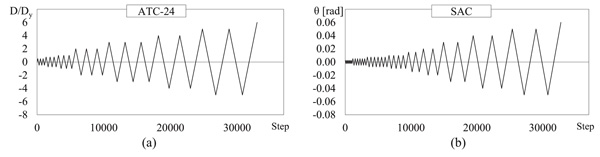
In this paper, two loading protocols are considered: the ATC-24 loading protocol [24] and the SAC loading protocol [25], which are depicted in Figs. (1a and b), respectively. The ATC-24 loading protocol was specifically proposed for the evaluation of seismic performance of components of steel structures. It assumes the yielding displacement Dy as the reference parameter for increasing the amplitude of cycles. The loading history is composed of at least six elastic cycles (i.e. with amplitude lower than Dy), followed by three cycles each of amplitude Dy, 2Dy and 3Dy, followed by pairs of cycles whose amplitude increases in steps of Dy until severe cyclic deterioration occurs.
The SAC loading protocol was developed based on a statistical study [27] performed on the number and amplitudes of storey drift cycles of two steel moment frames. This protocol adopts the storey drift angle rather than yielding deformation as the amplitude control parameter. Compared to the ATC-24 protocol, the SAC protocol contains smaller (elastic) cycles, two cycles of an intermediate amplitude, but slightly fewer cycles of larger amplitude. In particular, it is composed of three initial groups of cycles, which push the structure up to a storey drift angle equal to 0.0025 rad, 0.0050 rad and 0.0075 rad, respectively. Six loading cycles are included in each of those groups. The following four loading cycles lead the structure to a storey drift angle θ equal to 0.01 rad. The protocol concludes with further loading cycles that increase the storey drift angle attained in the previous loading cycle of 0.005 rad until failure.
2.2. Construction of the Backbone Curve
The base shear Vb versus top displacement Dt relationship obtained by the CPA is cyclic. To determine a single pushover curve that can be compared to that obtained by the monotonic pushover analysis, the cyclic response needs to be enveloped. To this end, the so-called backbone curve is determined according to the three following steps: (1) evaluation of the top displacement corresponding to the first yielding of the structure; (2) determination of the elastic branch; (3) determination of the plastic branch. In order to evaluate the yielding displacement Dy (step 1), the performance curve in terms of base shear and top displacement of the considered structure is required. To this end, a monotonic pushover analysis is run at first. In this paper, it was conducted by a distribution of lateral forces that is proportional to the first mode of vibration. Given the performance curve, the tangent stiffness is evaluated at each step. The top displacement corresponding to a tangent stiffness lower than 80% of the initial elastic stiffness is assumed as the yielding displacement Dy. As long as the structure is pushed towards a top displacement lower than Dy, the structure remains elastic. Thus, the elastic branch of the backbone curve (step 2) retraces the cyclic response. Since in a loading protocol several cycles are performed at a given amplitude of the displacement, it is necessary to identify for each considered amplitude of displacement Di the first loading branch and the first unloading branch in order to evaluate the following points of the backbone curve (step 3).

The points of the backbone curve following the yielding (step 3) are determined as the intersection between the first unloading branch of the cycles at amplitude Di-1 and the first loading branch of the cycles that go to a level of displacement Di larger than Di-1.
To clarify the procedure, Fig. (2) shows an example of the construction of the backbone curve. The SAC loading protocol applied in the CPA is shown in Fig. (2a) and the cyclic response is plotted in Fig. (2b) with the grey line. The first four groups of loading cycles of this loading protocol push the structure to top displacements lower than Dy, which is indicated by the dashed grey line in Fig. (2a). So far, the backbone curve (black line) follows the cyclic response (grey line), as shown in Fig. (2a). The following group of cycles pushes the structure to top displacements larger than Dy. For the sake of clarity, in this example, the top displacement equal to 0.594 m is considered. The red line in Fig. (2a) indicates the first unloading branch of this group of loading cycles. The cyclic response obtained during this unloading branch is plotted in red in Fig. (2b). The blue line in Fig. (2a), instead, identifies the first loading branch of the group of loading cycle that pushes the structure to a top displacement larger than that attained by the previous cycle (0.594 m), in this case, 0.693 m. The corresponding cyclic response is plotted in blue in Fig. (2b). The intersection between the unloading branch of the previous loading cycle (red line) and the loading branch of the following loading cycle (blue line) is the point of the backbone curve and is indicated by the grey dot. With this procedure, all the points of the backbone curve following the first yielding are obtained in Fig. (2b).
3. CASE STUDY BUILDING
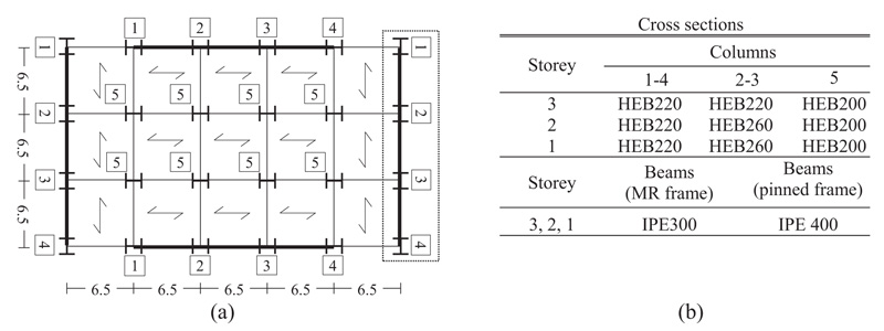
The case study building has been designed according to the provisions stipulated by EC8 [31] for steel moment resisting frames. The building has three storeys and the plan is rectangular-shaped (19.5 x 32.5 m2). The interstorey height h is 3.3 m and the mass at each storey is equal to 193.8 t. The structural scheme is composed of six three-span frames disposed along the longitudinal direction and four five-span frames along the transversal direction. Each span is 6.5 m long, as shown in Fig. (3). Columns are continuous in elevation and oriented as shown in Fig. (3a).
Both in X and Y directions, the seismic forces are sustained by the two three-spans external Moment Resisting (MR) frames (remarked in Fig. (3a) by a thick line). All the other frames are designed to sustain gravity loads only and thus beam-to-column connections are pinned. For the moment resisting frames, the design internal forces of the structural elements are the sum of those produced by the gravity loads included in the seismic design combination (denoted by subscript “G”) and those produced by the seismic forces (denoted by subscript “E”). The gravity load for the seismic design combination is equal to 6.0 kN/m2 and is determined considering characteristic values of dead and live loads equal to gk = 5.4 and qk = 2.0 kN/m2, and a combination coefficient ΨE equal to 0.3. In the non-seismic design combination, the sum of the vertical dead and live loads is equal to 10.56 kN/m2, assuming partial safety coefficients γg and γq equal to 1.4 and 1.5, respectively. The modal response spectrum analysis is applied to evaluate the internal forces due to the seismic action. To this end, the elastic response spectrum reported in EC8 for soil type A and scaled to a peak ground acceleration of 0.15 g is considered. In order to satisfy the code requirements both on strength of structural members at the ultimate limit state and on the storey drift at the damage limitation limit state, the behaviour factor is assumed equal to 5.
Beams are designed to have plastic moment resistance Mpl,Rd not lower than the design bending moment MEd. Furthermore, the cross sections are sized to prevent the decrease of plastic moment resistance and rotation capacity at the plastic hinge because of the design shear and axial forces. To this end, the relevant capacity design criterion is applied according to the following inequalities:
 |
(1) |
 |
(2) |
VEd,G, VEd,M and Vpl,Rd being the shear force in the beam due to the gravity loads, the shear force in the beam caused by the application of the moment Mpl,Rd of the beam with opposite sign at the two ending cross sections of the beam, and the shear resistance of the beam, respectively. Further, Npl,Rd is the plastic axial resistance and NEd is the design axial force.
As suggested by Elghazouli [32], the overstrength factor Ωmin of the beams of the frame is evaluated as the minimum of the following ratio in all the beams of the frame:
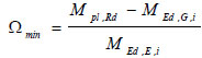 |
(3) |
Columns are designed to fulfil the resistance and stability verifications considering bending moment, axial force and shear force. The design values of bending moment, shear force and axial force are determined by the following relations:
 |
(4) |
 |
(5) |
 |
(6) |
These relations, which put into effect the capacity design for columns, do not apply for the evaluation of the design bending moment of the columns at the base of the frame and at the top level. Indeed, these internal forces are obtained from the structural analysis. In order to ensure sufficient local ductility, cross sections belonging to cross sectional class 1 are used for members devoted to yield.
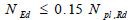
Since columns of the first storey frames are designed to be ductile, the following upper limits to their axial and shear forces are also considered:
 |
(7) |
 |
(8) |
Vpl,Rd and Npl,Rd being the plastic shear and axial resistances, respectively.
For the interior frames with pinned connections, columns and beams are designed to sustain gravity loads only and the adopted cross sections are HEB 200 and IPE 400, respectively.
4. SEISMIC ASSESSMENT OF THE CASE STUDY FRAME
To investigate the effectiveness of the CPA, the seismic response of the designed steel frame has been evaluated into two steps. First, the structural response of the case study building has been determined by nonlinear static methods of analyses, i.e. the CPA and the MPA. Both analyses have been run by applying forces distributed along the height of the frame proportionally to the first mode of vibration. From the monotonic performance curve (base shear Vbversus top displacement Dt), the yielding values of Vb,y and Dt,y are determined as those corresponding to a 20% reduction of the elastic stiffness. To investigate the influence of loading protocols on the seismic response, the CPA has been run twice, following the ATC-24 loading protocol and the SAC loading protocol. To compare the seismic response predicted by the CPA with that obtained by the MPA, the cyclic response obtained from each loading protocol has been enveloped by the corresponding backbone curve according to the procedure shown in section 2.2. For both the CPA and the MPA, the elastic spectrum proposed by EC8 for soil type C is used and each value of the displacement demand is associated with the corresponding peak ground acceleration (PGA) according to the Capacity Spectrum Method [7].
In the second step, the seismic response obtained by the CPA (with both loading protocols) and that evaluated by the MPA are compared with the structural response evaluated by the Incremental nonlinear Dynamic Analysis (IDA), assumed as the actual target response. To this end, artificial accelerograms, generated by the SIMQKE computer program [33, 34] and compatible with the assumed elastic response spectrum are used. The values of PGA are increased from 0.05 g to 1.20 g in steps of 0.05 g. A Rayleigh viscous damping is used and set at 5% for the first two modes of vibration. The stiffness coefficient of the Rayleigh formulation is applied to the tangent stiffness matrix of the elements. The second order effects are not included to avoid extra sources of degradation.
4.1. Numerical Model
The considered frame is three span wide and three storey high and it is the outermost one in the transversal direction (Fig. 3a). Beams and columns of the case study frames are modelled as beam with hinges elements. The middle part of the element is elastic, while the inelasticity is concentrated in the plastic hinge segments located at the two ends. Within the plastic hinge length, the cross section is subdivided into fibres.
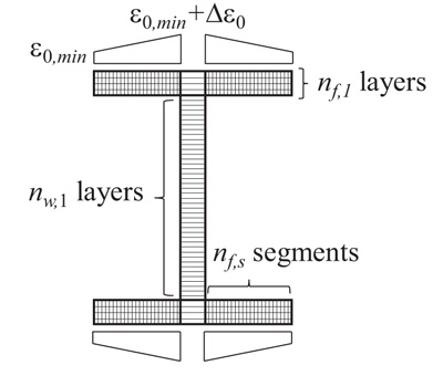
Because of the adopted design procedure, a significant inelastic behaviour is expected in beams while a moderate inelastic behaviour is expected in columns. For this reason, the degradation of stiffness and strength due to nonlinear cyclic behaviour is considered only for beams. Further, as reported in [35], the I-shaped cross section, commonly used for the MRF beams, starts deteriorating at the location of maximum bending moment due to the initiation of flange local buckling in the compression zone, which may also induce web deformation. Despite the interaction between flange buckling and web deformation, however the formation of local plastic mechanism at the level of flange in compression is a complex phenomenon and it leads to the general shape of the plastic mechanism. Instead, the local plastic mechanism for the web is sometimes partially formed. To simulate the degradation of stiffness and strength in beams due to local buckling of I-shape flanges, the numerical model proposed by Bosco and Tirca [23] is assigned to flange fibres of beam.
According to this model, each flange of the I-shape cross section is divided into nf,s segments and nf,l layers (30 x 4), while the web is discretized into nw,l layers (30), as depicted in Fig. (4). The uniaxial model by Menegotto and Pinto (Steel02) [36] is assigned to fibres in order to simulate the response of steel. According to this model, the relation that provides the normalised stress σ* as a function of normalised strain ε* is:
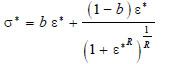 |
(9) |
where b is the strain hardening ratio assumed equal to 0.0030. The parameter R influences the shape of the transition curve and varies as a function of the plastic excursion ξpl of the previous loading path. It accounts for the Bauschinger effect and is updated in the analysis by the following equation:
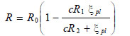 |
(10) |
Herein, R0 is the value of parameter R during the first loading, while cR1 and cR2 are experimentally computed. In the proposed model, the coefficient R0 is set equal to 20. Coefficients cR1 and cR2 are assumed equal to 0.925 and 0.15, respectively, as proposed in OpenSEES manual [37]. No isotropic hardening is considered. The yield strength Fy and the Young modulus E are equal to 235 MPa and 210000 MPa, respectively. This material model is able to take into account the accumulated plastic deformation at each point of load reversal. Accordingly, each hysteretic loop follows the previous loading path for a new reloading curve, while deformations accumulate. The low-cycle fatigue material is combined with Steel02 material assigned to fibres of the plastic hinge zones. The fatigue material (uniaxialMaterial Fatigue), which is already implemented in OpenSees, uses an accumulative strain model to predict damage in accordance with the Miner’s rule. The relationship between the plastic strain amplitude experienced at each cycle and the number of cycles to failure is that proposed by Coffin and Manson. The fatigue ductility exponent m is equal to -0.5. To simulate the gradual stiffness and strength degradation caused by local buckling, the fatigue coefficient ε0 is assigned to flange fibres according to a linear distribution [23]. In particular, a minimum value ε0,min is assigned to fibres located at the edges of both flanges and a maximum value (ε0,min + Δε0 ) is assigned to flanges fibres located at the intersection with the web (Fig. 4). The term ε0,min is related to the initiation of local buckling, and it is here assumed equal to 0.029, according to the value suggested in [23]. The term Δε0 controls the rate of degradation. Particularly, high values of Δε0 imply smoother stiffness and strength degradation, while low values lead to a more abrupt reduction of stiffness and strength. The value of Δε0 can be calculated according to the following equation given in [23].
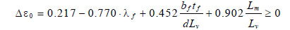 |
(11) |
d being the height of the cross section and λf the slenderness of the flange evaluated as function of Fy and E:
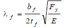 |
(12) |
In both equations (11) and (12), tf and bf are the thickness and the width of the flange, respectively. The shear length Lv and the wave length of beam flange during local buckling Lm are evaluated as follows [23]
 |
(13) |
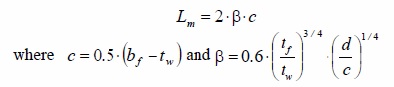 |
(14) |
tw being the thickness of the web. Finally, the length of the plastic hinge is set equal to 0.22 Lv [14].
No degradation is considered for cross sections of columns. In fact, capacity design principles are applied in design and columns sustain a minor yielding during earthquake. Thus, it is possible to consider a significantly lower number of fibres for the cross sections of these members. In particular, five fibres are considered for each flange and five fibres for the web. Four additional fibres are considered to simulate the root fillets.
4.2. Definition of the Seismic Input for Nonlinear Dynamic Analysis
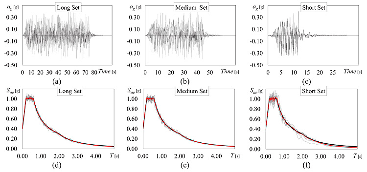
To consider a wide range of ground motion durations [33], three sets of ten artificial accelerograms generated by the computer program SIMQKE [34] were adopted as seismic inputs. Each accelerogram is defined by stationary random process modulated by means of a compound intensity function [38]. The earthquake rise time is 5.0 s, the parameter IPOW of the first branch and the parameter ALFA0 of the third one are assumed equal to 2.0 and 0.25, respectively. The stationary phase is followed by a latter 15 s phase with decreasing values of accelerations. Details regarding the envelope intensity function and the procedure for the determination of the length of the parts of the compound function may be found in [38]. The three sets are hereinafter named Long Set (LS), Medium Set (MS) and Short Set (SS). Each accelerogram of LS, MS and SS set is characterized by a total duration Tt equal to 90 s, 60 s and 27 s, and a duration of the stationary part Ts equal to 70 s, 40 s and 7 s, respectively. Figs. (5a, b and c) show an acceleration time history for each set. For each accelerogram, the value of the Arias Intensity AI has been calculated according to the following equation.
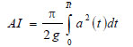 |
(15) |
where a is the ground acceleration recorded at each time step t. The significant duration of each ground motion, denoted as 5-95% Ds, has been determined as the interval between the times at which 5% and 95% of the Arias Intensity of the ground motion have been recorded, i.e. the duration of time over which the 90% of the energy is accumulated [22]. Given the values set for the total duration and the stationary part duration, the mean value of 5-95% Ds over the ten accelerograms resulted to be equal to 63.5 s, 37 s and 7.5 s for LS, MS and SS sets, respectively. These values are selected so as to cover the range of effective durations as reported in [22].
The accelerograms of each set are compatible with the elastic response spectra reported in EC8 for an equivalent viscous damping ratio equal to 5%, PGA equal to 0.35 g and soil type C. The elastic spectra of the selected accelerograms (grey thin lines), the corresponding average response spectra (red line) and the elastic spectrum of EC8 (black thick line) are shown in Fig. (5).
4.3. Parameters for the Evaluation of Seismic Response
The seismic response of the case study frame has been determined both in terms of global and local response parameters.
The assessment of the structural response at global level has been conducted considering the value of base shear Vb, top displacement Dt and peak ground acceleration (PGA). In the case of IDA, the value of every response parameter has been determined as follows. For every level of PGA and for each of the 10 ground motions, the maximum value of the relevant parameter during the time history is recorded. For each PGA, the mean value of the considered response parameter is calculated by averaging the values of the 10 ground motions. Consequently, every value of PGA corresponded to a value of Dt and Vb.
In the case of MPA, each point of the pushover curve (i.e. each couple of top displacement demand Dt and base shear Vb) is associated with the corresponding peak ground acceleration (PGA) according to the Capacity Spectrum Method [7], whereby the equivalent damping ratio ξeq is evaluated by the equation proposed for steel members in [39].
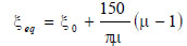 |
(16) |
where ξ0 is the inherent viscous damping, here assumed equal to 5%, and μ is the ductility demand evaluated at each step as the ratio of the displacement demand at the considered step over the yielding displacement Dt,y.
When the CPA is considered, instead, the Capacity Spectrum Method [7] is adopted with reference to the backbone curve.
The seismic response at local level was evaluated based on the distribution of storey drift along the height of the frame. In order to investigate a structural behaviour that ranges from the almost elastic to the strongly inelastic, two limit states were considered in the IDA, i.e. the attainment of a maximum storey drift equal to 2% and 6%. Each limit state corresponds to a value of peak ground acceleration (PGA2% and PGA6%) and top displacement ( ). Fixing the top displacement at the value corresponding to the attainment of the considered limit state in the IDA, the corresponding distribution of storey drift obtained by the IDA has been compared with that evaluated by the CPA and the MPA when either
  or
or  . In particular, in the case of the CPA, the top displacement
  corresponding to the drift limit state in the IDA was picked from the cyclic analysis, not the backbone curve.
Further, the seismic response has been investigated at cross section level. To this end, the values of bending moment M and curvature χ allowed the evaluation of the degradation of stiffness and strength in beams. In particular, the damage of the beams is measured by means of a damage index DI computed for each cross section within the plastic hinge zone of each I-shape beam. The DI is computed as the ratio of the number of flanges fibres in which the Miner’s damage index is equal to one (i.e. the number of fibres reaching fatigue) to the entire number of flange fibres within a given cross section [23]. When DI = 1.0, flanges of I-shape beam’s cross section are not able to contribute to the plastic resistance of the cross-section in the plastic hinge zone. A value of DI = 0.375, that corresponds to 80% of remaining bending moment capacity of the beam, was assumed to indicate the beam’s failure due to low-cycle fatigue [23]. In the case of the CPA, the DI is evaluated at the end of each loading cycle corresponding to the attainment of the top displacement imposed by the adopted loading protocol. For the sake of clarity, suppose that every top displacement Dt prescribed by the loading protocol is attained by a loading cycle composed of 5 loading branches. The number of damaged fibres is counted at the end of each loading branch. Then, once the fifth loading branch is completed, all the fibres that damaged after each loading branch are summed and the DI is evaluated. Instead, in the IDA the DI is evaluated at the end of the each time-history (i.e. of each accelerograms scaled at a given PGA). The obtained values of the DI of each cross-section are averaged over the number of accelerograms and are related to the maximum top displacement for the selected PGA. In order to have a comprehensive view of the damage in the frame, the following parameters were evaluated: (1) the average DIn evaluated at each n-th storey as the average value over the ending cross sections of the beams of the n-th storey, (2) the DIav evaluated as the average of the DIn over the n storeys; (3) the DImax evaluated as the maximum DI over the entire frame. The three response parameters were evaluated by the IDA and compared to those obtained by the CPA. No damage index can be evaluated when the MPA is carried out because there is no cyclic loading.
5. SEISMIC RESPONSE OF THE DESIGNED FRAME AND VALIDATION OF THE CPA
The seismic assessment of the designed steel frame aimed to (i) investigate the influence of the loading protocol and the influence of the rate of degradation on the seismic response predicted by the CPA, (ii) compare the effectiveness of the CPA to that of the MPA and (iii) validate the CPA through the comparison with the results obtained by the IDA.
5.1. Influence of the Loading Protocol on the Seismic Response Determined by CPA
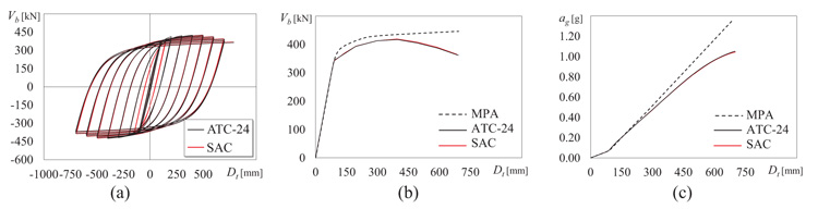
Fig. (6) compares the seismic response predicted by the CPA considering two different loading protocols, namely the SAC loading protocol (red line) and the ATC-24 loading protocol (black continuous line). The cyclic responses thus obtained are plotted in terms of base shear and top displacement in Fig. (6a). In Fig. (6b) the backbone curves corresponding to the cyclic responses obtained by the two loading protocols are plotted alongside with the performance curve obtained by the MPA (black dashed line). For each value of top displacement demand, the corresponding peak ground acceleration is determined by means of the Capacity Spectrum Method in Fig. (6c). Despite the different loading sequences and the different control parameter, the two loading protocols (SAC and ATC-24) lead to almost the same backbone curve (Fig. 6b). Since the backbone curves provided by the application of the two loading protocols are extremely close, the differences in the values of the peak ground acceleration corresponding to a fixed top displacement demand are negligible as well (Fig. 6c). The comparison between the results obtained by the MPA and those by the two cyclic pushover analyses show that, given a value of top displacement, the MPA leads to larger values of both base shear and peak ground acceleration compared to the CPA. This is due to the fact that the MPA is not able to take into account the effect of the cumulated damage, that is considered by the CPA, and neglects the corresponding reduction of stiffness and strength caused by the damage.
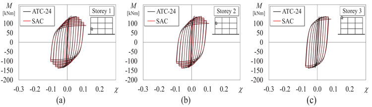
To examine the results more accurately, the seismic response is investigated at cross section level. Fig. (7) shows the bending moment M – bending curvature χ cyclic response of the left end cross section of the first span beam of the three storeys. Each M-χ loop is determined by the CPA applying both the considered loading protocols until the final top displacement. The stiffness and strength degradation of the cross sections is larger at lower storeys. Indeed, the cyclic response of the first storey is characterised by a larger loop than the third storey. The same tendency is found also for the ending cross sections of the other beams. In particular, at the third storey all the cross sections, with the exception of the outermost cross sections of the left and right beams, remain elastic and the cyclic response is linear. However, regardless of the cross section, the response is almost independent from the applied loading protocol. To delve deeper the analysis on stiffness and strength degradation, Fig. (8) plots the value of the average damage index Dn at each storey (Fig. 8a), the average damage index Dav of the frame (Fig. 8b) and the maximum damage index Dmax of the frame (Fig. 8b). Each of the damage indexes is evaluated at the attainment of every peak top displacement required by both the loading protocols. The dashed line is the threshold corresponding to the damage of 80% of fibres of the cross section, i.e. the failure of the considered cross section. At the end of the two loading protocols, i.e. for a top displacement equal to 693 mm and 700 mm for SAC and ATC-24 protocols respectively, the cross section that reached the largest damage index was the left end cross section of the first span beam of the first storey, where the DI was equal to 0.508 and 0.525, respectively. The largest mean Dn was recorded at the first storey and, at the end of the loading protocol, was equal to 0.496 for SAC protocol and 0.515 for ATC-24 protocol. The threshold value of DI was overcome at the second storey, as well. Instead, at the third storey the DI was on the average significantly lower than 0.375. At the end of the loading protocols, the average and the maximum indexes of the frame reached values equal to 0.319 and 0.508 for the SAC protocol, and 0.332 and 0.525 for ATC-24 protocol. According to the results presented so far, the differences in the seismic response due to the loading protocol are basically negligible. This is due to the fact that the two protocols differ mainly for the number of loading cycles in the elastic range, while the differences in the loading sequences in the inelastic range are negligible. Thus, the rate of degradation due to the cumulated damage is almost the same for both the loading protocols. Hence, the results by the CPA that will be discussed in the following paragraphs are only those obtained by the SAC loading protocol.
5.2. Influence of the Rate of Degradation on the Seismic Response Determined by CPA
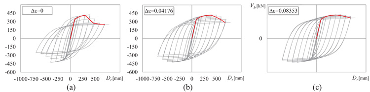
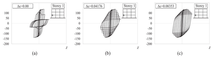
The fibre-based damage accumulation model introduces the parameter Δε to control the rate of degradation. This type of modelling allowed the investigation of the effect of the rate of degradation on the seismic response. To this end, the seismic response of the case study steel frame has been determined by the CPA considering three numerical models with values of Δε equal to 0.08353, 0.04176 and 0.0. The first value is provided in [23] based on the analysis of experimental results, and it is here assumed as the reference value. The second and the third values are selected to show clearly the changes in the structural response due to a reduction of Δε to 50%, or even to zero. The cyclic responses in terms of base shear and top displacement of the considered numerical models are shown in Fig. (9), whereby the corresponding backbone curves are plotted as well. Until the attainment of a top displacement approximately equal to 300 mm (i.e. 3% of interstorey height), the damage due to the cumulated fatigue has not occurred yet and the differences among the three backbone curves are almost negligible. After this value of top displacement, stiffness and strength tend to decrease almost simultaneously in each curve. Indeed, the degradation has occurred and some fibres, or even some cross sections, have collapsed. However, the reduction of stiffness and strength, denoted by the softening branch in the backbone curve, is related to the value of Δε. The value of Δε=0.0 represents the lower limit case. In fact, it makes the distribution of the fatigue coefficient ε0 constant along the flanges of the cross sections (Fig. 4). Hence, the damage occurs in all the fibres of the flanges simultaneously and the web of the considered cross section is the only resisting part. In this case every cross section can experience only two opposite scenarios: the entire cross section is effective (before the damage) or only the web is effective (after the damage the flanges suddenly collapse). Because of this, the moment resistance drops from that of the entire cross section to that provided by the web; for instance, Fig. (10a) shows the cyclic response of the left end cross section of the first span beam. This behaviour of the cross sections is reflected on the global response, which is denoted by the abrupt reduction of stiffness and strength shown in Fig. (9a). On the contrary, when Δε=0.08353 the fibres of the flanges collapse progressively. Thus, in addition to the two possible scenarios listed above, a third intermediate scenario could develop in the cross sections, i.e. the flanges are partially effective, because after the damage occurs only some fibres have collapsed, and the web is still effective. For this reason, the reduction of the moment resistance is very soft (see the example of the M- χ loop in Fig. (10c) and the slope of the backbone curve decreases smoothly, as shown in Fig. (9c). When Δε=0.0416, the behaviour is intermediate between those two limit cases.
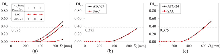
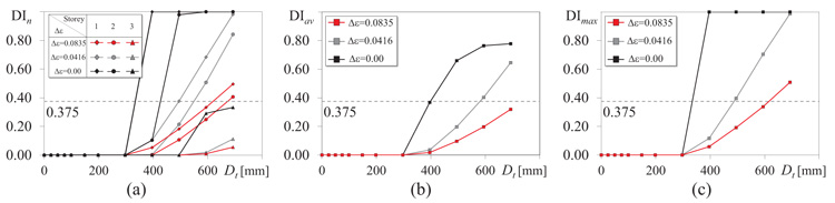
At cross section level, the rate of degradation affects the evaluation of the damage index as well. Indeed, when Δε is null, all the fibres of the flanges collapse simultaneously and the DI of a generic cross section can assume two alternative values: zero (before the damage) or 1 (after the damage), and the increase is abrupt. If Δε is larger than zero, the DI gradually increases from zero to 1, and the larger Δε the smoother the increase. Figs. (11a, b and c) show the average DIn at each storey, the average DIav and the maximum DImax, respectively. In these plots, the red, grey and black lines refer to the results obtained by assuming Δε equal to 0.08353, 0.0416 and 0.00, respectively. Fig. (11a) shows that the largest values of DIn are recorded at first and second storey, pinpointed by diamonds and dots, respectively. Regardless of Δε, the damage occurs at a top displacement equal to 300 mm. However, when Δε is null (black line) the average DIn index rises from zero up to (almost) 1 abruptly, while the increase of DIn is softer when Δε is larger than zero. Note that, given a value of the top displacement, the larger Δε the smaller the number of the collapsed fibres, thus the smaller DIn. Only at the third storey (pinpointed by triangles) the cross sections do not fail and DIn is below the limit value of 0.375. Nevertheless, also in this case the most sudden increase of DIn is attained when Δε is null. The same tendency is confirmed by the average DIav (Fig. 11b), and the maximum DImax (Fig. 11c) over the entire frame. It is worth noting that the value assumed for the rate of degradation influences the evaluation of the structural response. Indeed, a rough fibre discretization of the cross sections and a null value of Δε leads to an overestimation of the cumulated damage and an underestimated stiffness and strength. Instead, a fibre modelling able to consider the damage accumulation properly, i.e. with Δε larger than zero, allows a more accurate prediction of the effect of the cumulated damage on the structural performance. Based on these results, the following results are presented assuming Δε equal to 0.08353.
5.3. Effectiveness of the CPA and Validation
In this section the effectiveness of the CPA is evaluated by comparing the seismic response of the case study frame determined by the CPA with those obtained by the MPA and IDA, the last being assumed as the target response.
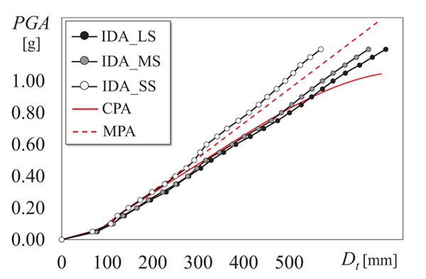
Fig. (12) shows the seismic response of the designed frame in terms of PGA and top displacement. The red continuous line and the red dashed line plot the results provided by the CPA (SAC loading protocol and Δε=0.08353) and MPA, respectively. A preliminary comparison between the two nonlinear static analysis shows that, for fixed values of PGA, the MPA leads to lower top displacements than the CPA. Indeed, the MPA neglects the effect of the cumulated damage, thus it is not able to account for the corresponding reduction of stiffness and strength. In the same plot, the three dotted lines show the maximum top displacement evaluated by the IDAs. The black, grey and white dots show the results obtained by the Long Set (LS), Medium Set (MS) and Short Set (SS), respectively. Particularly, for each of the three input sets, given the PGA, the corresponding top displacement is the average of the 10 maximum top displacements of the 10 accelerograms. The comparison of these three plots shows that the duration of the input accelerograms affects the seismic response. In fact, given a value of PGA, the SS leads to top displacements significantly lower than those attained under the MS or the LS. Thus, as long as the effective duration of the input accelerogram is short (7.5 s), the stiffness and strength degradation due to the cumulated damage is not significant. On the contrary, when the effective duration of the seismic input becomes significant (37 s and 63.5 s), the degradation of the cross sections turns into a critical issue. Based on these results, the CPA becomes extremely effective when accelerograms of medium or long duration are considered. In such cases, instead, the MPA would underestimate the top displacement demand. Instead, if short inputs are considered, the MPA is able to provide a reasonable prediction of the seismic response.
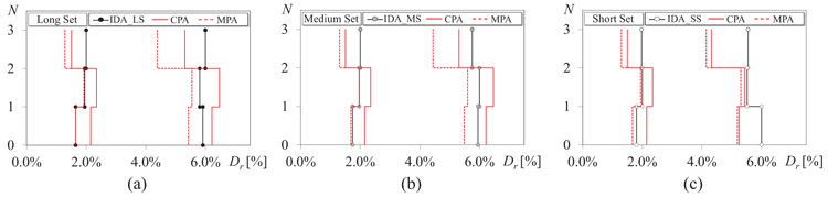
Figs. (13a, b and c) compares the heightwise distributions of storey drifts evaluated by the CPA and the MPA with those provided by the IDA with the long, medium and short input sets, respectively. For each set of accelerograms, the storey drift related to the IDA is the mean of the maximum values obtained by the 10 ground motions. Two limit states are considered in every IDA: the attainment of a maximum storey drift angles equal to 2% and 6%. The corresponding distributions of storey drifts of the CPA and the MPA are those corresponding to a top displacement equal to that leading the IDA to the considered limit state. At 2% limit state, regardless of the input set, the CPA overestimates the drifts of the first two storeys and underestimates that of the third storey, while the MPA provides a better estimation of the drifts at lower storeys, but underestimates, even more, the drift at the top storey. However, both the analyses indicate correctly the storey where the drift concentration is larger (second storey). When 6% limit state is achieved and the input set has long or medium duration, the CPA still provides a conservative estimate of the drifts, while the MPA significantly underestimates the storey drifts at every storey. Only in the case of the short set, CPA and MPA lead to almost equal drift estimates. However, also in this case the CPA is slightly more accurate than the MPA.
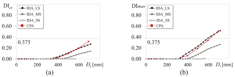
To validate the CPA at local level, Fig. (14) compares the average DIav and the maximum DImax of the entire frame evaluated by the CPA to the values provided by the IDAs with LS, MS and SS. The damage indexes DIav and DImax are calculated as described in Section 4.3. In both cases, the SS (white dots) has led to almost no damage in any cross-section and the average and the maximum DI are null. The largest damage is attained when the duration of the input is 90 s (black dots), in accordance with-the results shown in the previous figures. In this case, the damage index keeps a value on average lower than 0.375, owing to the beams of the third floor that basically remain elastic and decrease the average damage index. Instead, the maximum value of the damage index overcomes the limit value, due to the concentration of damage that cause failure of the beams of the first and second floors. The average and the maximum damage indexes estimated by the CPA (red line) are plotted along with those of the IDAs. This shows that the CPA is able to estimate accurately both the average and the maximum damage index caused by long duration accelerograms, in agreement with the results obtained in terms of global response parameters.
CONCLUSION
This paper uses the Cyclic Pushover Analysis to take into account a critical consequence caused by the cyclic character typical of earthquake loading, i.e. the degradation of stiffness and strength due to the damage cumulated in the cross sections. To investigate the CPA, a steel moment resisting frame was designed and modelled in OpenSees adopting a fibre-damage accumulation model. The seismic response of this frame was determined by the CPA following two loading protocols: the loading protocol proposed by SAC and the one proposed by the ATC-24. The effectiveness of the CPA was (1) examined through comparison with the conventional monotonic approach and (2) validated with reference to incremental nonlinear dynamic analyses. The IDA was conducted considering three sets of input accelerograms with short, medium and long duration. From the numerical analysis conducted on this model the following conclusions can be drawn:
- − Despite the differences between the SAC and the ATC-24 protocols, the seismic response of this frame determined by the CPA following two loading protocols led to almost the same structural response, with very negligible differences.
- − Based on the comparison between CPA and MPA, the CPA showed the capability of catching the stiffness and strength degradation, which is otherwise neglected by the MPA. In fact, given a base shear or peak ground acceleration, the CPA leads to the estimation of larger displacement demands compared to the MPA, which is consistent with the degrading processes that develop in the structural members.
- − During long (or medium) duration earthquakes, the cross sections of structural components undergo several loading cycles. Indeed, the IDAs show that, given a peak ground acceleration, the displacement demand is significantly larger than that caused by short duration earthquakes. Thus, the CPA was necessary to estimate accurately the response of the structure, particularly in the case of long duration earthquakes. In fact, at a PGA equal to 1 g, the CPA estimated the top displacement demand with an error lower than 10%, while the MPA underestimated it by 18%.
- − The importance of considering the cyclic deterioration is shown at local level, by means of the average and the maximum damage index of the frame. In the case of long earthquakes, given a top displacement of 600 mm (corresponding to a PGA equal to 1 g), the CPA estimated the damage indexes with an error equal to 12%.
To broaden the applicability of the CPA as a tool for seismic assessment, further studies will delve into the influence of the properties of loading protocols and the effect of the type of soil (rigid soil, soft soil) on the effectiveness of the CPA. Further analysis will be conducted on an extended set of case study frames, to investigate if the structural properties (geometrical properties, mechanical properties, presence of dissipative elements) affect the response predicted by the CPA.
CONSENT FOR PUBLICATION
Not applicable.
FUNDING
None.
CONFLICT OF INTEREST
The authors declare no conflict of interest, financial or otherwise.
ACKNOWLEDGEMENT
Declared none.