All published articles of this journal are available on ScienceDirect.

A Harbor Resonance Numerical Model with Reflecting, Absorbing and Transmitting Boundaries
Abstract
Background:
A very important aspect in the planning and design of a harbor is to determine the response of the harbor basin to incident waves. Many previous investigators have studied various aspects of the harbor resonance problem, though correct to a certain extent, have some disadvantages.
Objective:
To calculate wave response in an offshore or coastal harbor of arbitrary shape, this research develops a two-dimensional linear, inviscid, dispersive, hybrid finite element harbor resonance model using conservation of energy approach. Based on the mild-slope wave equation, the numerical model includes wave refraction, diffraction, and reflection. The model also incorporates the effects of variable bathymetry, bottom friction, variable, full or partial absorbing boundaries, and wave transmission through permeable breakwaters.
Methods:
Based on the mild-slope wave equation, the numerical model includes wave refraction, diffraction, and reflection. The model also incorporates the effects of variable bathymetry, bottom friction, variable, full or partial absorbing boundaries, and wave transmission through permeable breakwaters. The Galerkin finite element method is used to solve the functional which was obtained using the governing equations. This model solves both long-waves as well as short-wave problems. The accuracy and efficiency of the present model are verified by comparing different cases of rectangular harbor numerical results with analytical and experimental results.
Results:
There said results indicate that reduction in wave amplitude inside a harbor caused by energy dissipation due to water depth, linearly sloping bottom, and bottom friction is quite small for a deep harbor. But for a shallow harbor, these factors are critical. They also show that reduction in wave amplitude inside a harbor due to boundary absorption, permeable transmission, harbor entrance width, and horizontal dimensions.
Conclusion:
Those factors are very important for both deep and shallow harbors as proven by accurate agreement with the prediction of this numerical model. The model presented herein is a realistic method for solving harbor resonance problems.
1. INTRODUCTION
Groups of linear and nonlinear waves with high crest pose hazards to ships, inducing harbor resonance and over-topping of structures. In the planning and design of a harbor the response of the harbor basin to incident waves is crucial but modelling of waves varies dramatically. A harbor is dynamically similar to a mechanical or acoustical system, where certain wave oscillation phenomena may produce resonance. Numerous studies have been conducted on various aspects of the harbor resonance problem. Lee [1] developed a theory for wave-induced oscillations in constant depth harbors of arbitrary geometry, by applying Weber’s solution of the Helmholtz equation. Chen and Mei [2, 3] developed a linear inviscid, nondispersive, hybrid finite element model based on a variation principle for treating arbitrary platform geometries. Houston [4] used a model based on the mild-slope equation to study the interaction of tsunamis with the Haeaiian Islands. Zelt [5] derived a Lagrangian description of nonlinear, dispersive and dissipative processes for wave propagation in two horizontal dimensions, to study the influence of sloping boundaries on the long wave response of bays and harbors. Tsay et al. [6, 7] and Hamidi et al. [8] applied the mild-slope equation to effects of topographical variation and energy dissipation. Ganaba, et. al. [9] and Woo, et. al. [10, 11] developed finite element methods for boundary layer modelling with application to dissipative harbor resonance problems. Boussinesq equation models have also been successfully applied to harbor modelling (Abbott and Madsen, 1990) [12]. These previous numerical model studies have contributed significantly to the understanding of harbor resonance, but have not included wave energy dissipation with bottom friction, boundary absorption and wave transmission through permeable breakwaters. Researchers took advantage of rapid growth of computation capacity of computer to further develop tools analysing long waves [13, 14] and nonlinear waves [15, 16].
Analytical investigation results also showed that the boundary conditions greatly affect the harbor resonance. Many research programs focused on the harbor depths from constant slope [16, 17], Cosine squared bottom [18], exponential bottom [19], to parabolic bottom [20] and geometric configuration [21], and the singular boundary method (SBM) [22] (ISBM) [23]. Therefore, the need to develop realistic and fully interactive models for the prediction of wave conditions inside a basin is imperative.
In the present study, the governing model equation is based on the mild-slope wave equation, including wave refraction, diffraction and reflection, and the effects of variable transmission through permeable breakwaters. The function is based on a conservation of energy approach which represents the physical characteristics of actual harbors in a realistic environment. An effective hybrid finite element method is used for solving the mild-slop wave equation. The entire harbor basin is divided into a number of triangular finite elements. The resulting wave amplitudes response at the node points is matched with the eigenfunction expansion employed for the region outside the harbor. The sensitivity of the present model is evaluated by comparing the numerical results with analytical and experimental results for different cases of rectangular harbors.
2. THEORETICAL DEVELOPMENT
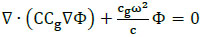
In this theoretical development, the fluid is assumed homogeneous, inviscid, incompressible, and its motion irrotational. Berkhoff [24] derived an expression for two-dimensional, monochromatic waves of infinitesimal amplitude, over slowly varying water depths, which modelled both refraction and diffraction. The resulting mild-slope wave equation can be expressed as:
 |
(1) |
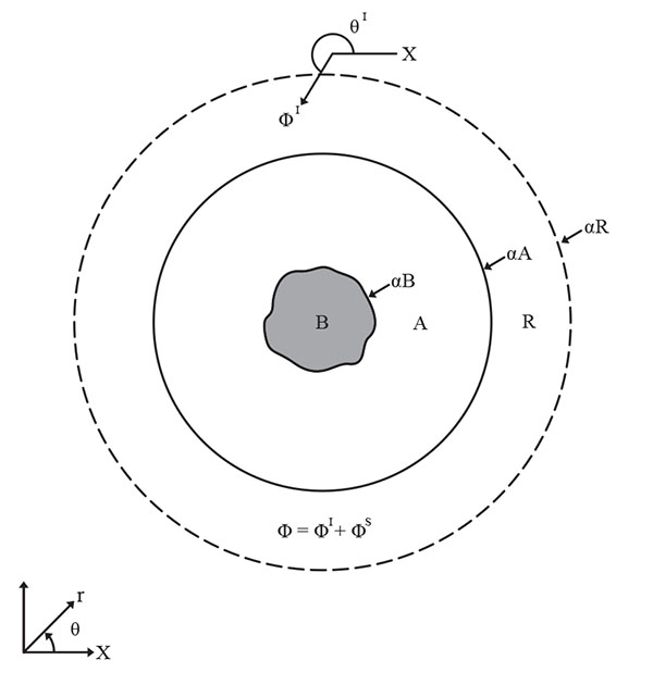
where Φ (x, y) is the velocity potential on the mean free surface z = 0 and the vertical variation in the potential is: 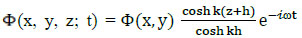 , and c = ω/k is the phase velocity, which can be calculated from the dispersion relation ω2 = gk tanh kh and Cg = dω/dk is the group velocity, where k is the wave number, ω is the radian frequency, and h is the water depth.
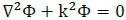
If water depth is constant or deep, Eq.(1) reduces to the Helmholtz equation:
 |
(2) |
2.1. Arbitrary-Shape Harbor Formulation Governing Equation
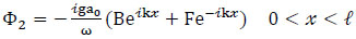
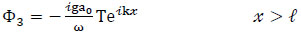
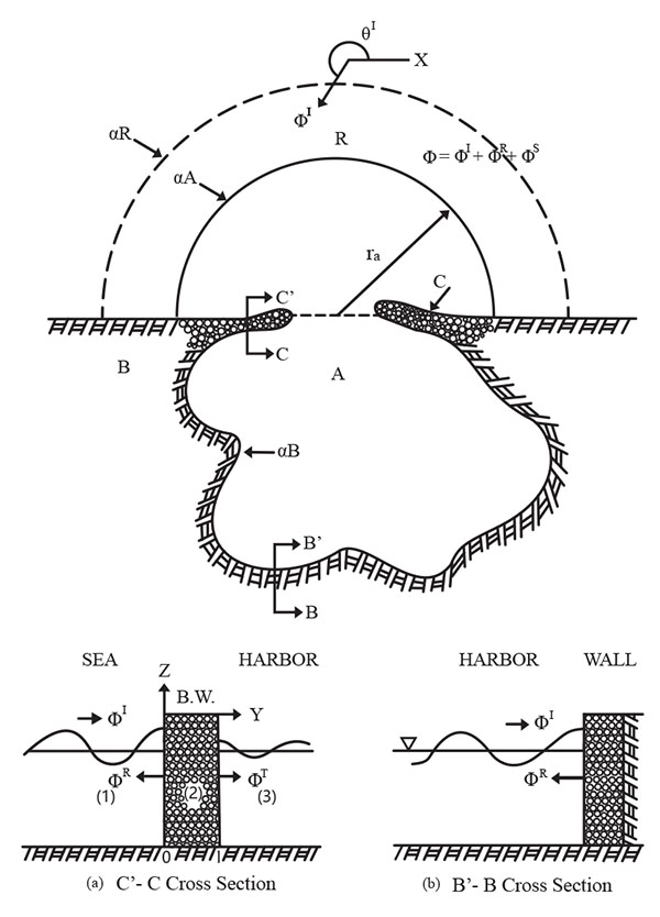
For an arbitrary-shape harbor, the domain is divided into two regions as shown in Fig. (1): Region A is the limit of the harbor and Region R is the infinite open-sea. ∂A is near island region as shown in Fig. (1), and also in the harbor basin region shown in Fig. (2), ∂C is the breakwater boundary shown in Fig. (2). The governing equations for the respective regions can be expressed as:
 |
(3) |
and
 |
(4) |
Where, water depth is constant or deep.
The total velocity potential can be separated into incident (ΦI), reflected (ΦR), and scattered (ΦS) wave potentials, such that Φ = ΦI + ΦS (for offshore harbor), and Φ = ΦI + ΦR + ΦS (for coastal harbor).
The incident wave potential can be expressed as:
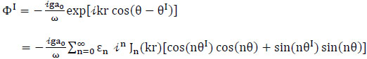 |
(5) |
where ε0 = 1, εn = 2, n = 1, 2…. are the Neumann factors, a0 is the amplitude of incident waves, θI is the incident angle, Jn is the Bessel function of the first kind and order n, θ is the angle variable in polar coordinates, and r is the radial coordinate.
For a semi-infinite ocean with a straight coastline, the reflected wave potential can be written as:
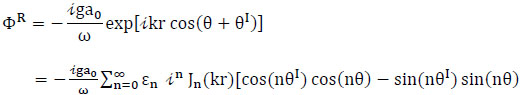 |
(6) |
The scattered wave potential satisfies the Helmholtz equation and Sommerfeld radiation condition, which can be written as:
 |
(7) |
where Hn1 is the Hankel function of the first kind of order n, αn and βn are unknown coefficients yet to be determined. The boundary conditions fall into the following domains:
(1) The domain B (Fig. 1) represents the harbor, along whose boundaries appropriate boundary conditions must be specified. On a solid boundary, the normal velocity must vanish, i.e. ∂Φ/∂n = 0, where n is the outward normal vector to the boundary.
In practical problems, reflection may be partial where energy absorption occurs. Therefore, the general boundary condition can be represented as:
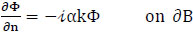 |
(8) |
Where, α is a boundary absorbing coefficient that must be empirically prescribed.
(2) In the infinite sea region R, the boundary ∂R is taken as a circular or semicircular contour. A Sommerfeld radiation condition is imposed at infinity in all horizontal directions and the scattered wave ΦS must be an outgoing wave at infinity:
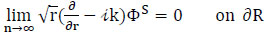 |
(9) |
(3) A matching continuity condition is imposed along the boundary that may be expressed as:
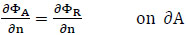 |
(10) |
 |
(11) |
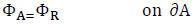
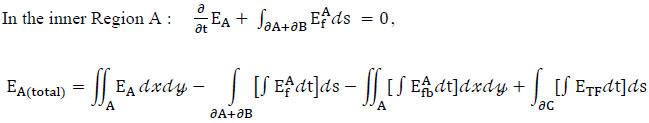
2.2. Conservation of Wave Energy Formulation
The present method derives a function from the principle of conservation of energy. The total wave energy in the inner Region A,EA (total), is the sum of the total wave energy in Region A,(EA) energy loss from boundary absorption dissipation (Ef), bottom friction energy loss (Ebf), and energy transmission through the permeable breakwater (ETf), which may be expressed as:
 |
(12) |
In the outer Region R: 
So the total wave energy can be expressed as:
 |
(13) |
For a progressive long wave, the average total energy may be obtained from the contributions of both potential energy (PE) and kinetic energy (KE).
(1) The potential wave energy for per unit wave length is:
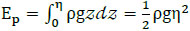 |
(14) |
where ρ is the water density, g is the acceleration due to gravity, and 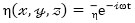 . The mean free surface is located at z = 0 and the free surface elevation η can be derived from the linearized Bernoulli’s equation and the dispersion relation as:
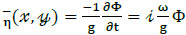 |
(15) |
Substituting Eq.(15) into (14), the simplified potential wave energy equation is:
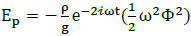 |
(16) |
(2) The kinetic wave energy for per unit wave length is:
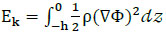 |
(17) |
where the velocity potential is given as  , the velocity potential for monochromatic waves with angular frequency ω, is
 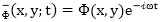 . Substituting into Eq.(17) results in:
 |
(18) |
Then the simplified kinetic wave energy equation is:
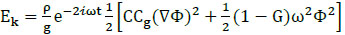 |
(19) |
where 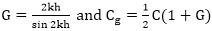 .
.
Total wave energy is equal to potential (Eq.16) and kinetic (Eq.19) components, expressed as:
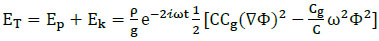 |
(20) |
2.3. Wave Energy Flux
The instantaneous energy flux of a progressive long wave passing through a section of unit width, characterized by its horizontal normal n, can be expressed as:
 |
(21) |
where P is the complex excess pressure,  , and Uc is the complex particle velocity in the normal direction,
  ; then,
 |
(22) |
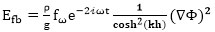
2.4. Bottom Friction
A portion of wave energy dissipation is caused by bottom friction. Bottom energy flux per unit area (Efb) can be expressed as:
 |
(23) |
where Ub is the instantaneous particle velocity at the bottom.
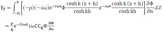
Conventionally the shear stress is defined as:
 |
(23a) |
where (τb,max) real and (Ub,max)real2 and kb are the real-valued maximum shear stress, potential theory particle velocity, and wave friction at the bottom, respectively. Jonsson [25]
For convenience, we define:
 |
(24) |
where  and has dimensions of ft2/sec3
Particle velocity at the bottom (Ub) can be expressed as:
 |
(25) |
 |
(26) |
Substituting Eqs. (24) and (26) into Eq. (23) results in a bottom friction energy flux equation:
 |
(27) |
 |
(27a) |
2.5. Absorbing Boundary
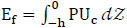
The wave partial reflection due to wave energy dissipation at the absorbing boundaries may exist such as the instantaneous wave energy flux at the absorbing boundaries. EfA is the instantaneous wave energy flux, measured positive, from A out through ∂B to ∂A. One can integrate the instantaneous energy flux as Eq.(22) with respect to time then yield:
 |
(28) |
Because of the absorbing boundary condition Eq.(8),  , then along the absorbing boundaries ∂B can be written as:
 |
(29) |
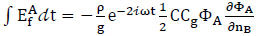
2.6. Transmission Through Permeable Breakwater
Permeable harbor structures, such as rubble-mound breakwaters, have been widely constructed to provide protection from wave attack by reflecting and dissipating incident wave energy. At a permeable breakwater only part of the incident wave energy is reflected back to the ocean, while the rest is absorbed and/or transmitted into the harbor through the structure. If this transmitted energy is exceedingly high, it may create undesirable and unsafe wave conditions inside the harbor.
Consider a two dimensional interaction of a monochromatic wave train with a single homogeneous, isotropic, porous structure of width located between two semi-infinite fluid regions, as shown in Fig. (2). The damping region occupies 0 < x < l and the flow domain extends to infinity (x → ± ∞). The wave field can be divided into three regions:
Region 1: x < 0, Energy dissipation can occur (incident wave region)
Region 2: 0 < x < l, Energy dissipation can occur (absorbed and transmitted wave region)
Region 3: x > l, No energy dissipation (transmitted wave region)
Since the solution in adjacent regions must be continuous at each interface, the appropriate boundary conditions are the continuity of pressure and horizontal mass flux at y = 0 (between region 1 and 2) and y = l (between region 2 and 3), expressed as,
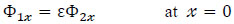 |
(30) |
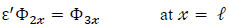 |
(31) |
where ε, ε' are the porosity of the porous medium, the solution of the velocity potential in each region (similar to Liu, et. al. [26]) can be written as:
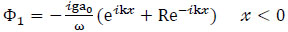 |
(32) |
 |
(33) |
 |
(34) |
where a0 is the incident wave amplitude, B and F are unknown constants to be determined, R is the reflection coefficient, and T represents the transmission coefficient.
The wave transmission through a porous structure, such as the instantaneous wave energy flux at Region 3 (Fig. 2), can be written as:
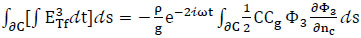 |
(35) |
From Eqs. (32) and (34), assuming that Φ3 = kTΦI, results in,
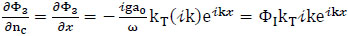 |
(36) |
where ΦI is the incident wave potential, and kT is an empirical transmission coefficient, Eq.(35) can then be written as:
 |
(37) |
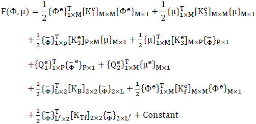
2.7. Construction of a Functional F (Φ)
Combining total wave energy (Eq.20), bottom friction (Eq.27), absorbing boundary (Eq.29), and transmitting boundary (Eq.37) terms, a functional can be obtained from Eqs.(12) and (13) such that, the stationary functional is then:
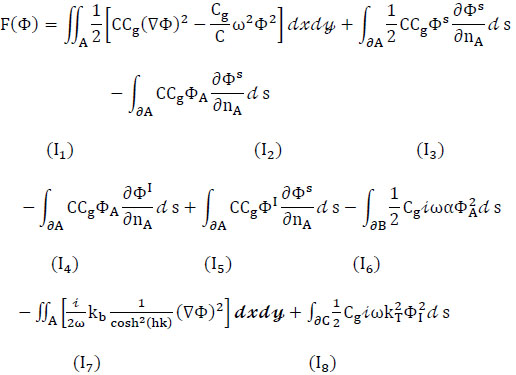 |
(38) |
The discretization of terms I1 to I8 will be discussed in detail in the following section.
3. FINITE ELEMENT NUMERICAL FORMULATION
The hybrid finite element method used to solve the mild-slope wave equation is similar to the one developed by Chen and Mei [2] for shallow-water wave problems. The entire harbor basin is divided into a number of finite elements of triangular shape (in the finite inner region A). Wave amplitude at the nodal points is sought and the solution is matched with Eigen function expansion employed for the region outside the harbor (in the infinite outer region R).
3.1. Evaluation of the Functional
The interpolation function  is used to evaluate the functional, and the Gaussian quadrature four-point method of numerical integration is used to solve for phase velocity and group velocity. Using this approach the functional, Eq. (38), can be evaluated as follows:
(1) First term (energy in region A):
 |
(39) |
with
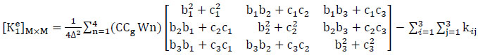 |
(40) |
where Wn is the weighting function, and 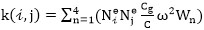
(2) Second term (energy flux along ∂A):
 |
(41) |
with
 |
(3) Third term (energy flux along ∂A):
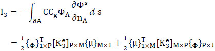 |
(42) |
with
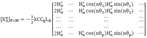 |
(42a) |
(4) Fourth term (energy flux along ∂A):
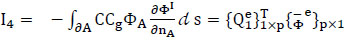 |
(43) |
with
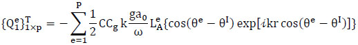 |
(43a) |
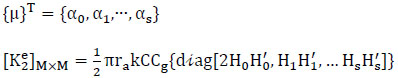
(5) Fifth term (energy flux along ∂A):
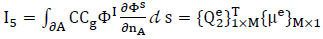 |
(44) |
with
 |
(44a) |
(6) Sixth term (boundary absorption energy flux along ∂B):
 |
(45) |
with
 |
(45a) |
where L is the total number of line elements along the inner boundary ∂B, LBe is the length of each segment, and α is a boundary absorption coefficient, dependent on empirical and laboratory data.
(7) Seventh term (bottom friction energy flux along A):
 |
(46) |
with
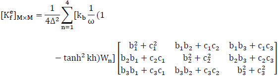 |
(46a) |
where Wn is a weighting factor and Kb is an empirical bottom friction coefficient.
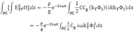
(8) Eighth term (energy transmitting through porous structures along ∂C):
 |
(47) |
with
 |
(47a) |
where L' is the total number of line elements along the porous structures (breakwater) ∂C, LC'e is the length of each segment, and kT is the transmission coefficient.
3.2. Assemblage and Extermination of the Functional
Assembling the local stiffness matrix into a global stiffness matrix results in the functional being written as:
 |
(48) |
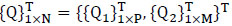
By combining nodal unknowns and coefficient unknowns and defining the total unknown vector {ϕ} by
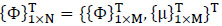 |
(49) |
where N=M+M and
 |
(50) |
the functional can be written as:
 |
(51) |
where the total load vector
 |
(52) |
and the total stiffness matrix [K] is usually large and banded,
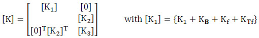 |
(53) |
then, the stationary functional of F(Φ) implies that
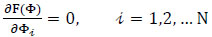 |
(54) |
Substitution of equation (54) into equation (51), leads to
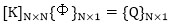 |
(55) |
This set of N linear algebraic equations for N unknowns can be solved by the LU elimination method. The total velocity potential at all nodal points and unknown coefficients can also be determined.
4. NUMERICAL EXAMPLES
For verification of the numerical model, a rectangular harbor has been tested for different cases as follows:
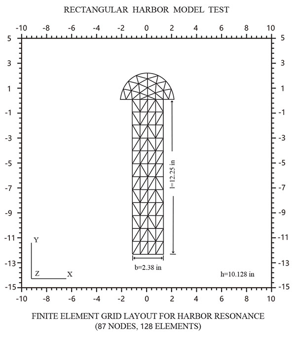
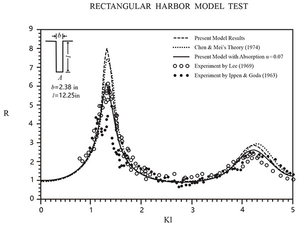
4.1. Fully-Open Rectangular Harbor
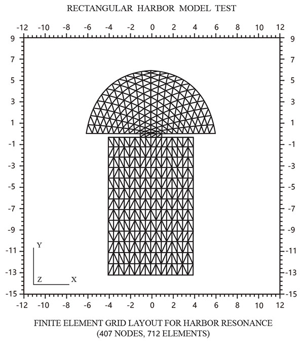
A fully-open rectangular harbor finite element grid layout is shown in Fig. (3). The present model results are compared with existing experimental data of Ippen and Goda [27], Lee [1], and Chen & Mei’s [2, 3] model, as shown in Fig. (4). The incident wave angle θI = -π/2 the present model with boundary absorption α = 0.07, bottom friction coefficient Kb = 0.3. The resulting curve is the most exact replica of the experimental results. It reveals an accurate agreement between the numerical results and experimental data.
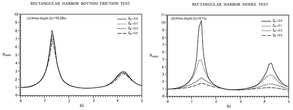
4.2. Bottom Friction Testing
Fig. (5) shows the effect of energy dissipation due to bottom friction. For deep harbor (h = 10.128 in.) case as shown in top Fig. (5), the reduction in wave amplitude inside the harbor is quite small; for shallow harbor (h=0.1 in.) case as shown in bottom Fig. (5), the wave response is quite sensitive.
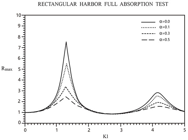
4.3. Full Boundary Absorption Testing
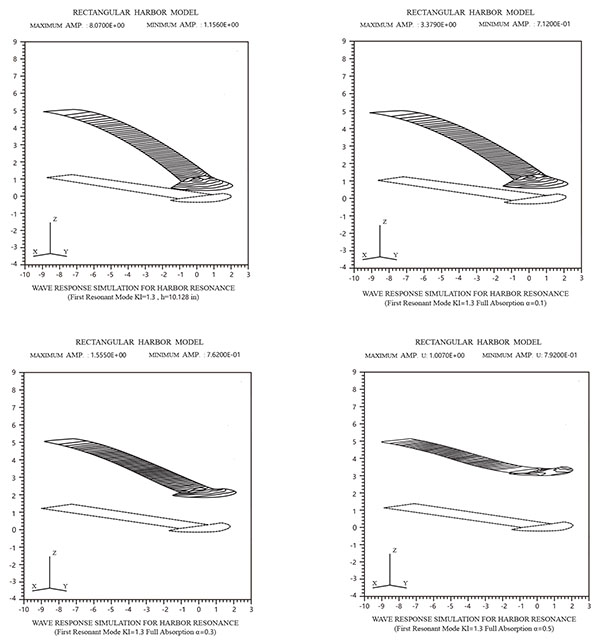
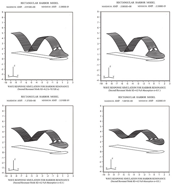
In order to test the effect of energy dissipation due to fully absorbing boundaries, as shown in Fig. (6), when the boundary absorption coefficient (α) increases, it shows an increase in the highly sensitive response curves reactively. In order to express more effectively using three-dimensional plots, Figs. (7 and 8) show a three dimensional plot of the relative surface elevations for the harbor resonance response of the first and second resonance mode, for the inner boundary absorption coefficients α equal to 0.0, 0.1, 0.3, and 0.5 respectively.
4.4. Partial Boundary Absorption Testing
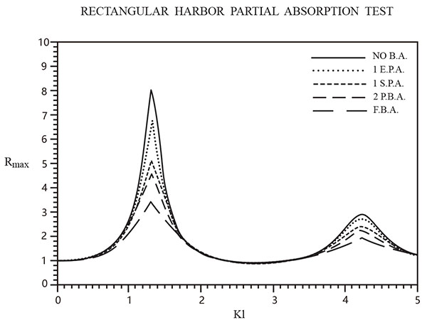
In a realistic harbor, which consists of breakwaters, quay walls, and wharfs, boundary reflection factors may be quite different. Fig. (8) shows the effect of partial boundary absorption (P.B.A.) on Rmax for five different boundary absorption conditions: (1) No boundary absorption, (2) One end wall with P.B.A. (4 elements, α = 0.3), (3) One side wall with P.B.A. (12 elements, α = 0.3), (4) One side and one end walls with P.B.A. (16 elements, α = 0.3), (5) All three walls with P.B.A. (27 elements. α = 0.3). The results seem reasonable and point to the fact that as the total area of absorption (i.e. number of absorbing boundary elements) increases, the harbor response should be reduced.
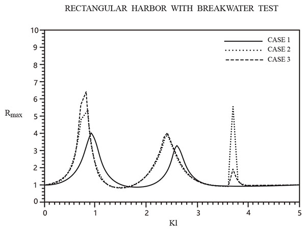
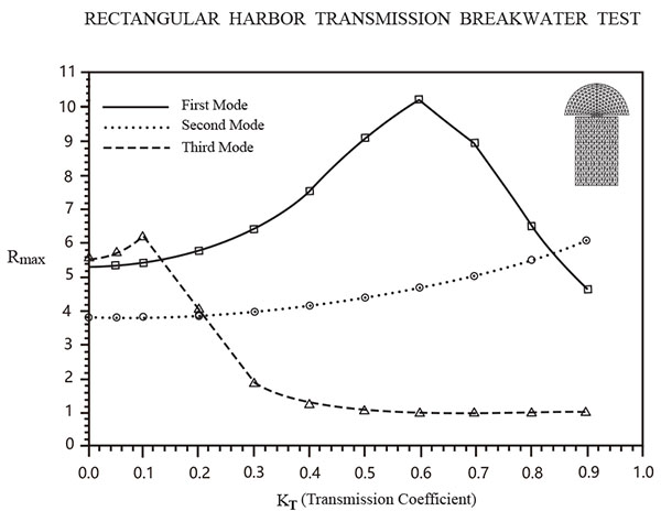
4.5. Permeable Transmitting Boundary Testing
A wider rectangular harbor with breakwater, with its finite element grid layout shown in Fig. (9) reveals the effect of permeable transmitting boundaries for three cases as shown in Fig. (10). The harbor with an impermeable breakwater creates a larger response as the energy inside the harbor can’t be reflected back to sea. Apparently a harbor with permeable breakwater has more energy flux transmitted through the porous structure into the harbor, and thus produces the largest response, even larger than that produced for a harbor with impermeable breakwater. Fig. (11) shows variation of maximum amplification (Rmax) with a different transmission coefficient (KT) for the first, second, and third resonant modes for a harbor with permeable breakwater. Larger amplification occurs for (KT) and smaller wave number (Kl). When KT is within the range 0.3 to 0.8, a larger amplification is produced in the first and second resonant modes.
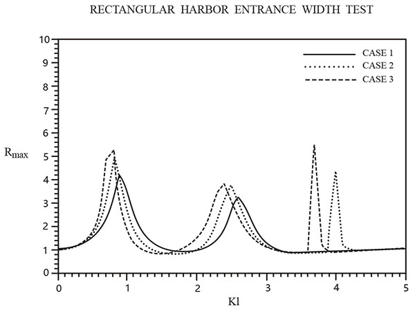
4.6. Variable Harbor Entrance Width Testing
Fig. (12) shows the effect of variable harbor entrance using three cases: (1) Fully open entrance, (2) Partial 4 inch entrance width, (3) Partial 2 inch entrance width. As the entrance width decreases, the response curve amplitude increases and Kl decreases. The model thus confirms the Harbor Paradox of Miles and Munk [28].
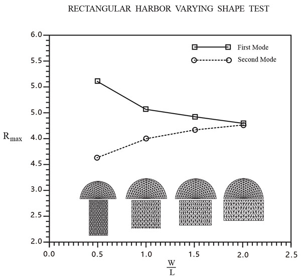
4.7. Varying Length and Width Testing
Fig. (13) shows the effect of varying length and width for a rectangular harbor with a constant basin area and entrance width, using four different horizontal dimensions. As the basin length decreases and width increases, the response curve amplitude for the second resonant mode increases and has a larger Kl.
CONCLUSION
A realistic harbor resonance model has been developed based on the conservation of wave energy principle. This approach was used to develop a two-dimensional linear, inviscid, hybrid finite element model for calculating the free surface response characteristics inside a harbor, subject to excitation by incident waves from outside the harbor. The numerical model is based on the mild-slope wave equation which includes wave refraction, diffraction, and reflection, under the effects of variable bathymetry, bottom friction, variable full or partial absorbing boundaries, and wave transmission through permeable breakwaters. The conservation of energy principle is intuitively appealing in describing harbor resonance, because of one of its uses of fundamental physical laws. The total wave energy in the harbor is a combination of kinetic and potential wave energy, and instantaneous wave energy flux. This flux consists of the effect of bottom friction dissipation, absorbing boundaries dissipation, and transmission through porous boundaries (which increases available energy). This approach is used to derive a stationary functional which is equivalent to the mild-slope governing equation and boundary conditions. Model calculations for a rectangular harbor support the following conclusions. Reduction in wave amplitude inside the harborsis important for shallow water harbors. Results showed that energy dissipation due to boundary absorption, permeable transmission, entrance width, and horizontal dimension are very important for both deep and shallow water harbors. In order to improve model response prediction results, more experimental work is needed to better determine values for absorption and transmission coefficients.
NOMENCLATURE
| Phase velocity | c | ||
| Group velocity | cg | ||
| Wave energy | E | ||
| Bottom friction energy loss | Ebf | ||
| Energy flux rate | Ef | ||
| Boundary absorption energy dissipation | (Ef)∂B | ||
| Kinetic wave energy | Ek | ||
| Potential wave energy | Ep | ||
| Energy transmission through permeable breakwater | ETf | ||
| Functional | F(Φ) | ||
| Bottom friction coefficient | kb | ||
| Shoaling factor, defined by Eq.18 | G | ||
| Gravitational acceleration | G | ||
| Water depth | H | ||
| Bessel function | Jn | ||
| Wave number (2π/wave length) | k | ||
| Transmission coefficient | kT | ||
| Length of each segment | L | ||
| Excess pressure | P | ||
| Radial coordinate | r | ||
| Particle velocity | Uc | ||
| Bottom wave velocity | Ub | ||
| Weighting function | Wn | ||
| Horizontal coordinates | x,y | ||
| Vertical coordinate | z | ||
| Coefficients of eigenfunctions | αn,βn | ||
| Jacobi symbols | εn | ||
| Spatial factor of free surface displacement | η | ||
| Angle variable in polar coordinates | θ | ||
| Water density | ρ | ||
| Bottom shear stress | τb | ||
| Velocity potential | Φ | ||
| Radian frequency | ω | ||
| near island boundary | ∂A | ||
| Inner boundary | ∂B | ||
| Porous structure breakwater boundary | ∂C | ||
| Vector formed by α_n,β_n | {μ} | ||
| Vector formed by nodal potential | {ϕ} | ||
| Total unknown vector | {Φ} | ||
| Superscripts | Subscripts | ||
| Element | e | Region A | A |
| Incident | I | Region R | R |
| Radiation | R | Incident | I |
| Scattering | S | Index | i , j |
| Transmission | T | Transmission | T |
CONSENT FOR PUBLICATION
Not applicable.
CONFLICT OF INTEREST
The authors declare no conflict of interest, financial or otherwise.
ACKNOWLEDGEMENTS
This study was funded by The Southeast Coastal Engineering Structure Disaster Prevention and Reduction of Engineering Research Center of Fujian Province Program (No. JDGC03) and The natural sciences Research Foundation of Putian University (No. 2015074).