All published articles of this journal are available on ScienceDirect.

A Simplified Method for Determining the Bearing Capacity of Eccentrically Compressed Rectangular CFST Columns with Eccentricities in Two Planes
Abstract
Introduction
Rectangular concrete-filled steel tubular (CFST) columns are among the most promising types of load-bearing structures. Compared to circular CFST columns, they are more effective in resisting eccentric compression. Existing analytical calculation methods enable the determination of the bearing capacity of eccentrically compressed CFST columns in the presence of axial force eccentricity in only one plane. The purpose of this work is to develop an analytical method for calculating the bearing capacity of eccentrically compressed CFST columns in the presence of bending moments in two planes.
Materials and Methods
The proposed model is based on the theory of limit equilibrium. Four main variants of the neutral line location in the cross-section at the moment of destruction are identified. For each variant, resolving equations are obtained that allow for determining the ultimate load, which can be solved using the publicly available Microsoft Excel Online software.
Results
The developed method was tested on experimental data for 38 samples. The correlation coefficient between the experimental and calculated values was 0.979. There is also good agreement between the results of analytical calculations and the results of finite element modeling.
Discussion
The deviation of the experimental ultimate load values from the calculated ones can be attributed to the scatter of experimental data and the local loss of stability effects on the pipe wall.
Conclusion
Engineers can use the proposed method for a preliminary assessment of the bearing capacity for eccentrically compressed CFST columns at the stage of selecting design solutions.
1. INTRODUCTION
Concrete-filled steel tubular (CFST) columns are widely used in construction due to their high load-bearing capacity, seismic resistance, and cost-effectiveness. Their key advantage is the synergy of the steel shell and concrete core: steel provides ductility and tensile strength, while concrete demonstrates increased compressive strength [1]. This combination increases the load-bearing capacity and gives the columns pronounced dissipative properties, which is critically important for seismically hazardous regions [2-4].
Additional advantages of CFST columns include fire resistance, durability, and the ability to create slender structures without losing strength [5-8]. This is why CFST columns have become a popular choice for high-rise buildings, bridges, and other critical structures worldwide [9].
In their research, scientists consider issues of strength, deformability, and stability of CFST columns under central and eccentric compression, as well as under temperature loads, using experimental, numerical, and normative-analytical calculation methods [10].
Experimental studies, despite their high reliability, require significant financial and time resources, which limits their large-scale application. Since the first experiments conducted by Klöppel and Goder, numerous experimental studies of CFST columns with varying geometric and physical-mechanical characteristics have been carried out, primarily under axial loading, and less frequently under eccentric compression in a single plane [11-25]. The authors compare the experimental results with calculations using national standard methods. An analysis of 3103 CFST column tests previously showed that European and Australian standards provide more accurate but conservative predictions [26]. However, their application beyond the established limits leads to less reliable results. Du et al. note that there are no experimental data available for rectangular columns made of high-strength steels with a yield strength exceeding 400 MPa, which necessitates additional research [27].
Despite the significant volume of experimental data, their fragmentation and lack of systematization make complex analysis and practical application difficult. Additionally, the limitations of testing equipment and the increase in construction scale do not allow for obtaining completely reliable results under various types of loading.
Numerical methods, particularly the finite element method, are widely employed to analyze the behavior of rectangular CFST columns, offering accurate modeling of nonlinear material properties, geometry, and contacts, as well as the impact of concrete lateral compression. The reliability of the obtained results is confirmed by the authors in papers, where the results correlate with calculations using standard methods [28-33].
Compared to circular columns, rectangular columns offer better coupling with beams under complex loading, demonstrating resistance to cyclic loads, which is particularly important in seismically hazardous regions [34, 35].
There are relatively few studies devoted to the analysis of eccentric compression with eccentricities in two planes for rectangular columns, as confirmed by a bibliometric network analysis of 783 scientific sources using VOSviewer software (Fig. 1) [36]. Most works consider CFST columns with compression and bending only in one plane.
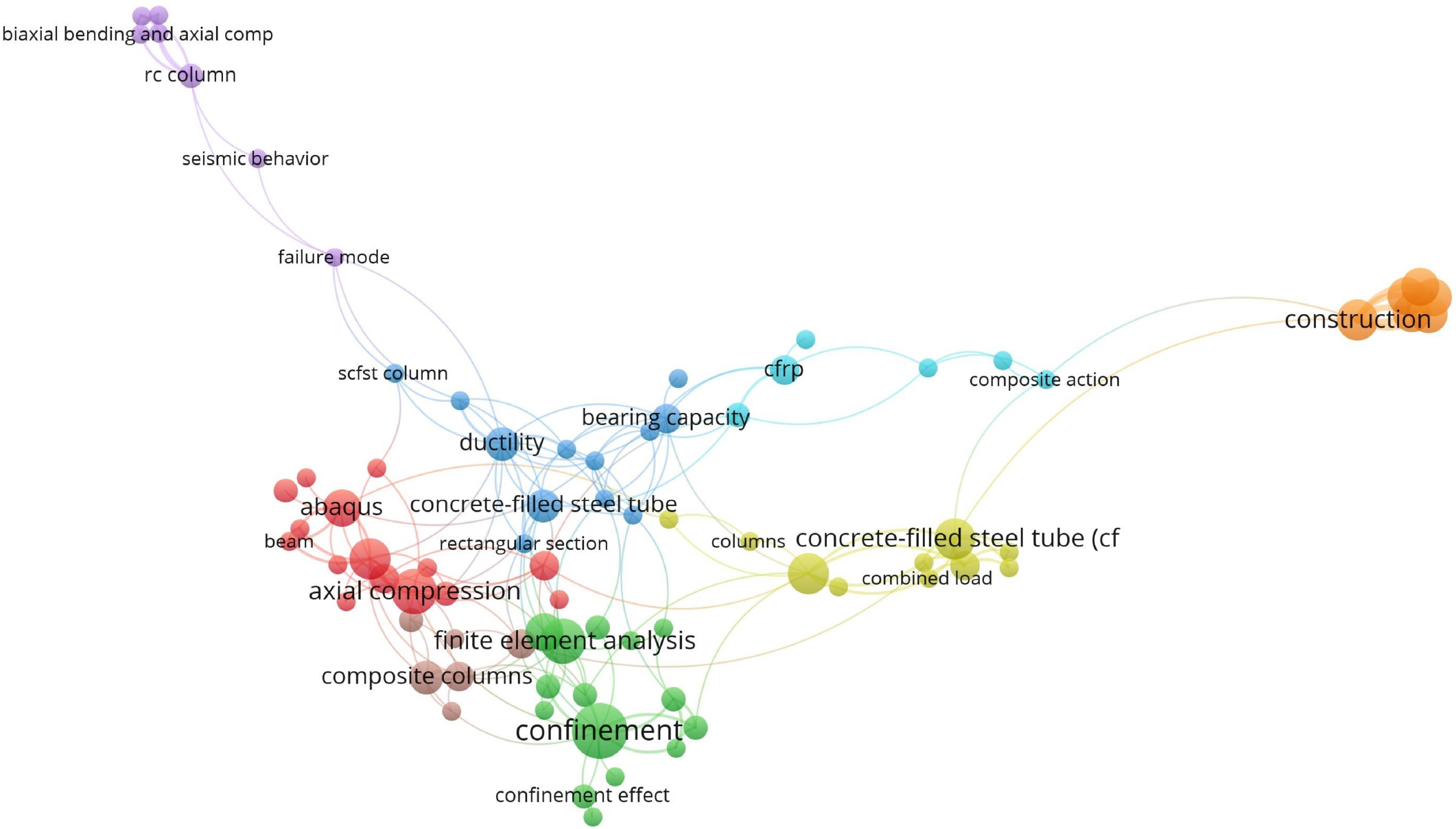
Bibliometric map of CFST column research.
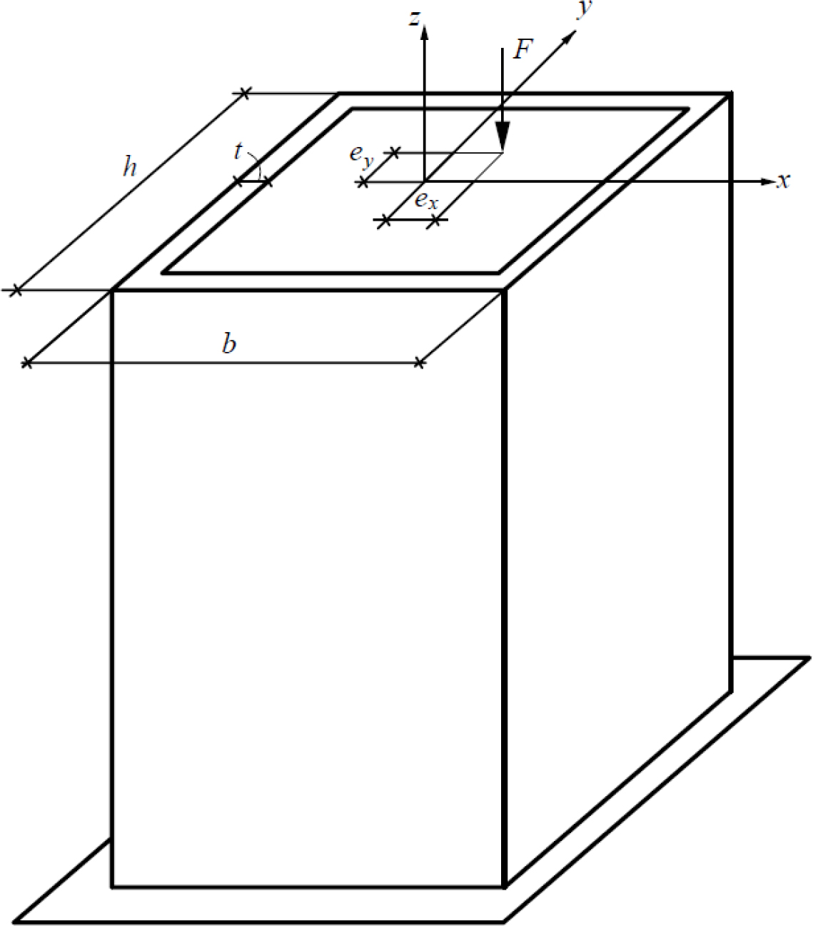
Calculation scheme.
Visualization of the key research areas thematic network revealed understudied areas, particularly the area of eccentric compression with eccentricities in two planes (biaxial bending and axial compression), which is represented on the knowledge map by a small cluster weakly connected to the main areas. This suggests that research in this area is being conducted, but its integration into the overall scientific agenda is limited: the main focus is on numerical analysis methods, while analytical models that take into account biaxial loading are practically underrepresented.
The conducted literature analysis confirms the relevance of the study, which aims to develop methods for assessing the strength of CFST columns operating under complex stress conditions. The purpose of this work is to develop a simplified analytical method for calculating the bearing capacity of eccentrically compressed CFST columns in the combined action of axial forces and biaxial bending. Such a method will allow engineers to obtain quick and well-founded solutions without the need to develop complex calculation models in software packages or perform labor-intensive experimental studies.
The article is structured as follows. The materials and methods section presents the main assumptions of the model, possible failure schemes, and the resolving equations for each scheme. The results and discussion section presents the testing of the proposed model using experimental data. A numerical example of calculation is also presented to enable the reproduction of the results by other researchers. In conclusion, the main findings of the work are presented.
2. MATERIALS AND METHODS
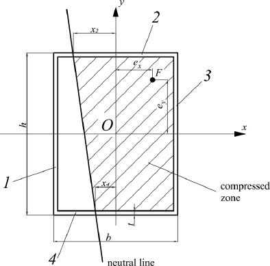
The calculation scheme of the considered structure, which is an eccentrically compressed rectangular CFST column experiencing compression with biaxial bending, is shown in Fig. (2).
The simplified method is based on the following assumptions:
1. The increase in compressive strength of concrete in a CFST element due to the effect of lateral compression is not taken into account.
2. The stress in the compressed zone of the concrete core in the limit state is constant and equal to the compressive strength of concrete Rb.
3. The stresses in the tensile zone of the concrete core are neglected.
4. The material of the steel shell is assumed to be ideal elastic-plastic, and in the limit state, the stresses in the tensile and compressed zones of the steel shell are equal to the yield strength of the steel Ry with the corresponding sign.
5. The neutral line, which divides the section into compressed and stretched zones, is the straight line in the limit state.
6. The dimensions of the concrete core are assumed to be approximately equal to the external dimensions of the column cross-section. That is, the wall thickness of the rectangular steel profile pipe is considered negligible compared to the cross-section dimensions.
7. The effects of local stability loss due to the pipe wall are neglected.
8. Additional eccentricities of the axial force caused by the deflection of the element are not taken into account.
Assumptions 2-5 are the standard hypotheses of the limit equilibrium method [37]. Hypothesis 8 implies that geometric nonlinearity is not considered in the calculation. Its consideration is well developed for the case of bending in one plane [38], but for biaxial bending, its consideration in the analytical model will cause great difficulties.
For convenience, we will assume that the point of application of the eccentric compressive force is located in the first quadrant of the coordinate system xOy. Depending on the relationship between the eccentricities of the axial force ex ey, seven cases are possible:
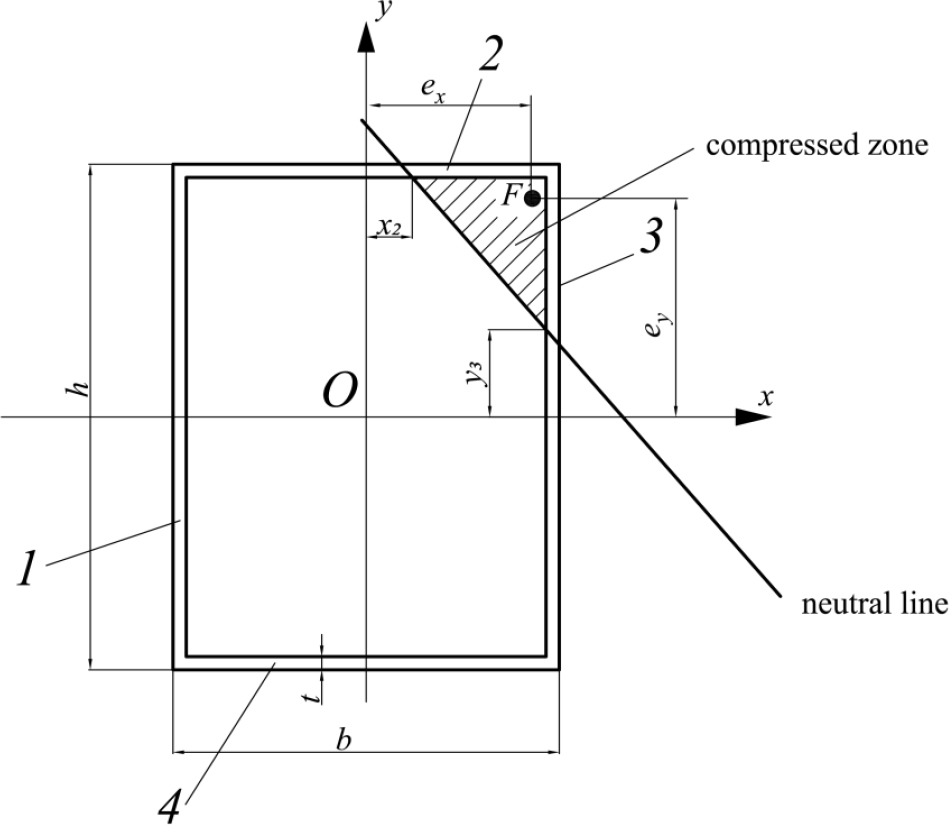
1) The neutral line intersects sides 1 and 3 of the cross-section contour (Fig. 3).
2) The neutral line intersects sides 1 and 4 of the cross-section contour (Fig. 4).
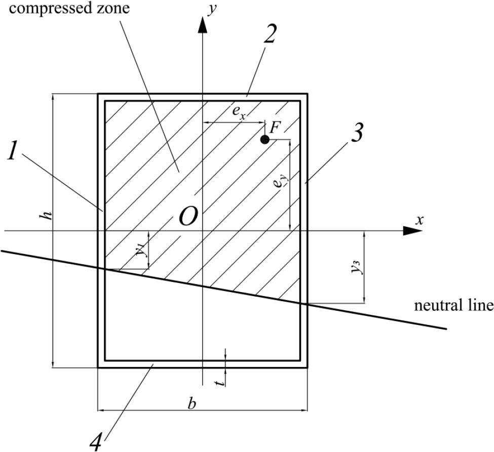
Option 1 of the neutral line position.
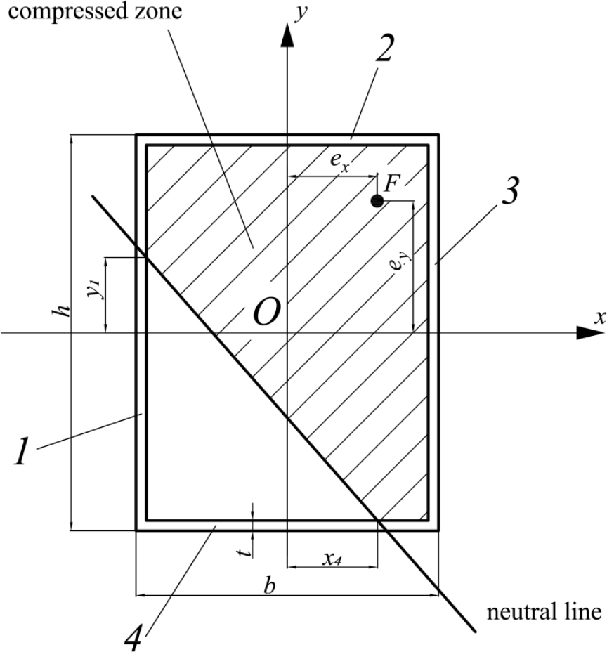
Option 2 of the neutral line position.
3) The neutral line intersects sides 2 and 4 of the cross-section contour (Fig. 5).
4) The neutral line intersects sides 2 and 3 of the cross-section contour (Fig. 6).
Option 3 of the neutral line position.
Option 4 of the neutral line position.
5) If one of the eccentricities of the axial force ex is equal to zero, then a case is possible when the compressed zone of concrete covers the entire concrete core, and only side 4 of the steel pipe works in tension (Fig. 7).
6) When ey = 0 and ex
 0 a case is possible, when only side 1 of the steel pipe is subject to tension (Fig. 8).
7) Case of axial compression ex = 0 ey = 0.
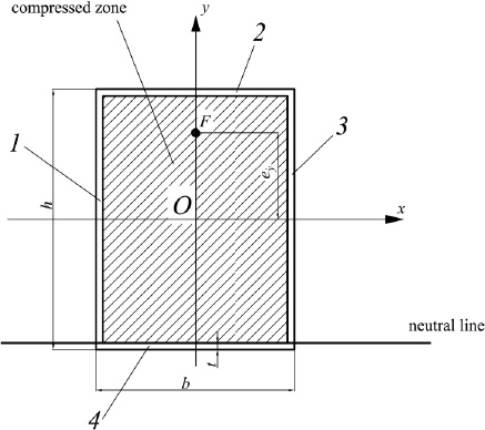
Option 5 of the neutral line position.
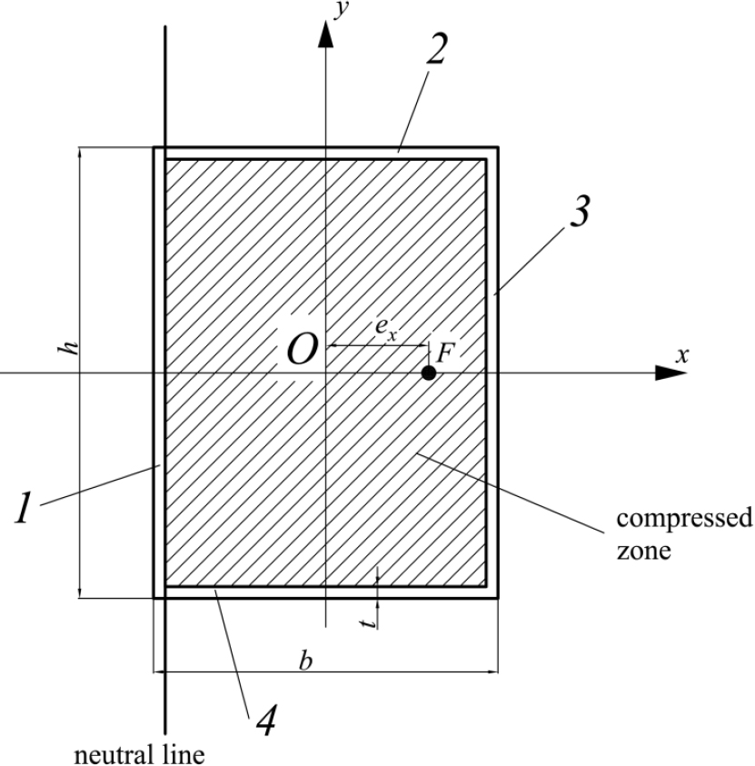
Option 6 of the neutral line position.
Let us begin by considering option 1. The following constraints must be met with this option for distances y1 and y3 according to Fig. (3) (Eq. 1):
 |
(1) |
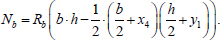
The axial compressive force perceived by concrete is the product of the concrete compressive strength Rb and the area of the concrete core compressed zone (Eq. 2):
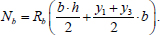 |
(2) |
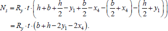
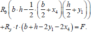
The axial compressive force perceived by the steel shell Ns is the product of the yield strength and the difference between the cross-sectional area of the compressed zone of the steel pipe and the tensile zone area. Ns value can be written as (Eq. 3):
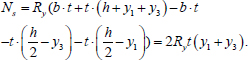 |
(3) |
The sum of the forces Nb and Ns gives the magnitude of the compressive force F (Eq. 4):
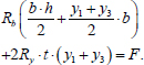 |
(4) |
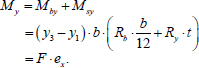
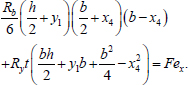
The bending moment about the axis y, perceived by concrete, represents the product of the compressive strength, the area of the compressed zone, and the coordinate of the compressed zone center of gravity. It is written as (Eq. 5):
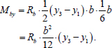 |
(5) |
The bending moment about the axis y, perceived by the steel shell, is determined as follows (Eq. 6):
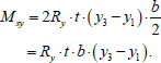 |
(6) |
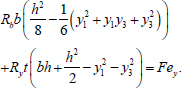
Based on Eqs. (5 and 6), the following equilibrium condition can be written (Eq. 7):
 |
(7) |
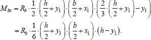
The bending moment about the axis x perceived by concrete is calculated as follows (Eq. 8):
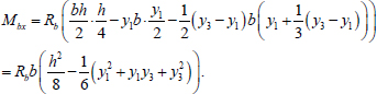 |
(8) |
The bending moment about the axis y, perceived by the steel shell, is calculated using the formula (Eq. 9):
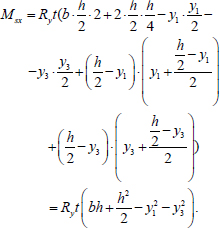 |
(9) |
Based on (Eqs. 8 and 9), the following equilibrium condition can be written:
 |
(10) |
Thus, the problem of determining the ultimate load for option 1 is reduced to three equations (Eqs. 4, 7, 10) with three unknowns y1, y3, F.
The three equations indicated can be reduced to a single equation with respect to F. To do this, we express the sum (y1 + y3) from Eq. (4), and we express the difference (y3-y1) from Eq. (7):
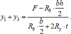 |
(11) |
 |
(12) |
Adding Eqs. (11 and 12), we obtain the formula for y3 (Eq. 13):
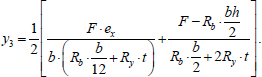 |
(13) |
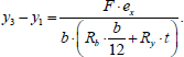
Subtracting Eqs. (12 from 11), we obtain the formula for y3:
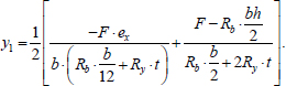 |
(14) |
Next, substituting Eqs. (13 and 14 into 10), we obtain a quadratic equation with respect to F. The roots of this equation must be substituted into Eqs. (13 and 14) and the fulfillment of conditions in Eq. (1) must be checked. The smaller positive value of F, at which conditions in Eq. (1) are satisfied, will correspond to the ultimate load. Failure to fulfill conditions in Eq. (1) or the absence of positive roots of the quadratic equation with respect to F indicates that the limit equilibrium is not realized according to option 1.
Option 3 (Fig. 5) is similar to option 1 (Fig. 3). The equilibrium equations for this option are written as (Eqs. 15-17):
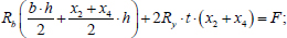 |
(15) |
 |
(16) |
 |
(17) |
From Eqs. (15 and 16), values x2 and x4 can be expressed through F in the following form (Eq. 18):
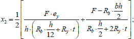 |
(18) |
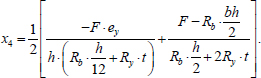 |
(19) |
Substituting Eqs. (18 and 19 into 17), we also obtain a quadratic equation with respect to F. After finding the positive roots of the equation, they must be substituted into Eqs. (18 and 19) and the conditions must be checked (Eq. 20):
 |
(20) |
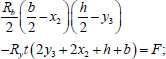
Let us consider option 2 (Fig. 4). The compressive force perceived by concrete will be written as (Eq. 21):
 |
(21) |
The axial force perceived by the steel shell is determined as follows (Eq. 22):
 |
(22) |
The first equilibrium equation takes the form (Eq. 23):
 |
(23) |
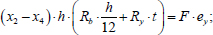
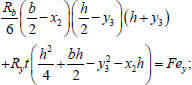
The bending moment about the axis x, perceived by concrete, is determined by the formula (Eq. 24):
 |
(24) |
The bending moment about the axis x perceived by the steel shell is calculated as follows (Eq. 25):
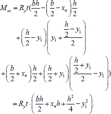 |
(25) |
The second equilibrium equation (the sum of the internal and external moments relative to the x-axis) is written as (Eq. 26):
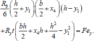 |
(26) |
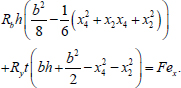
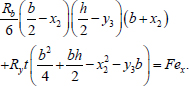
The equation for the sum of moments about the y-axis has a similar form (Eq. 27):
 |
(27) |
Thus, for option 2 (Fig. 4), the problem of determining the ultimate load is reduced to a system of three nonlinear equations (Eqs. 23, 26, 27) with respect to the variables y1, x4 and F. In this case, the following constraints must be satisfied for y1 and x4 (Eq. 28):
 |
(28) |
The nonlinear system of equations (Eqs. 23, 26, 27) has more than one solution. The problem of determining the ultimate load at failure, as per option 2, is formulated as a nonlinear optimization problem. The objective function, which is the compressive force F, as determined by Eq. (23), must reach a minimum. The constraints are determined by Eqs. (26-28). We have implemented the search for the ultimate load in the MATLAB environment using the interior point method [39].
Option 4 (Fig. 6) is similar to option 2 (Fig. 4). This option is possible in the case of large eccentricities of the axial force. The equilibrium equations for this option are written as (Eqs. 29-31):
 |
(29) |
 |
(30) |
 |
(31) |
The solution of system (Eqs. 29-31), as for option 2, is performed using nonlinear optimization methods. In this case, the following constraints must be satisfied for x2 and y3 (Eq. 32):
 |
(32) |
The impossibility of finding a solution that satisfies conditions (Eq. 32) or the negative value of the force F found indicates that the destruction does not occur according to option 4.
For option 5 (Fig. 7), the ultimate load is determined by the formula (Eq. 33):
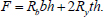 |
(33) |
An indication that option 5 is being implemented may be that, when calculating according to option 1, the values y1 = y3 turned out to be greater than h/2.
For option 6 (Fig. 8), the formula for the ultimate load has the form (Eq. 34):
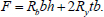 |
(34) |
An indication that option 6 is being implemented may be that when calculating according to option 3, the values x2 = x4 turned out to be greater than b/2.
For the case of axial compression (option 7), the formula for the ultimate load has the form (Eq. 35):
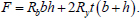 |
(35) |
3. RESULTS
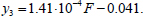
The developed methodology was tested on experimental data for 38 samples presented in three different works [40-42]. In Fig. (8), the experimental values of the ultimate load Nexp are plotted along the abscissa axis, and the values Ncalc calculated using the method proposed in this article are plotted along the ordinate axis. Most of the points are located fairly close to the straight line Nexp = Ncalc. A tabular presentation of the data shown in Fig. (9) is given in Table 1. This table also presents the results of the finite element calculation NFEM using the simplified method given in the paper [43], and the number of the destruction scheme (option) is indicated for each sample.
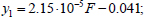
It should be noted that in recent works [41, 42], concrete compressive cube strength was given instead of the prismatic compressive strength. The following relationship (Eq. 36) was used to calculate prismatic (cylindrical) compressive strength Rb by the compressive cube strength R [44]:
 |
(36) |
4. DISCUSSION
As shown in Table 1, for samples HSS3 and HSS4, as well as HSS16 and HSS17, the same ultimate load values were obtained at different eccentricities of the axial force. This can be explained by the fact that at a small eccentricity, the neutral line can be inside the wall of the steel pipe. Since we considered the wall thickness to be small compared to the cross-sectional dimensions, this case was not considered. It turned out that for both columns, destruction occurs according to Scheme 6. It should also be noted that Uy tested two twin samples for some variants (HSS1 and HSS2, HSS8 and HSS9, HSS14 and HSS15) [40].
Statistical characteristics for the relationships Nexp/Ncalc and NFEM/Ncalc are presented in Table 2.
It is evident from Table 2 that the average values of the ratios Nexp/Ncalc and NFEM/Ncalc are close to one. The deviation of the values from the calculated values can be explained, in part, by the scatter of experimental data. In some cases, deviations can be explained by the presence of local loss of stability effects for the pipe wall (which leads to a decrease in the actual ultimate load compared to the calculated one). The other reason for deviations is an increase in the bearing capacity of the concrete core due to the effect of lateral compression (which leads to an increase in the actual ultimate load compared to the calculated one).
The values NFEM show a smaller deviation from the values Ncalc, since the finite element calculation excludes errors associated with the spread of material characteristics and the presence of random eccentricities. The correlation coefficient between the values Nexp and Ncalc was 0.979, and between the values NFEM and Ncalc it was 0.983.
For the possibility to reproduce the results, we also give a numerical example of calculation for the sample Rcfst-4 from Table 1 at b = 0.18 m, h = 0.12 m, t = 3∙10-3 m, Rb = 4.67 ∙ 104 kPa, Ry = 3.24 ∙ 105 kPa, ex = 0.036 m, ey = 0.024 m.
To determine the ultimate load according to option 1, we substitute the initial data into Eqs. (13 and 14). As a result, we obtain Eqs. (37 and 38):
 |
(37) |
 |
(38) |
Comparison of calculation results with experimental data.
| Sample | b, cm | h, cm | t, mm | Rb, MPa | Ry, MPa | ex, cm | ey, cm | Nexp, kN | NFEM, kN | Ncalc, kN | Scheme |
|---|---|---|---|---|---|---|---|---|---|---|---|
| Uy, 2001 [40] | |||||||||||
| HSS1 | 11 | 11 | 5 | 28 | 750 | 0 | 0 | 1836 | 1909 | 1989 | 7 |
| HSS2 | 11 | 11 | 5 | 28 | 750 | 0 | 0 | 1832 | 1909 | 1989 | 7 |
| HSS3 | 11 | 11 | 5 | 30 | 750 | 1.5 | 0 | 1555 | 1400 | 1188 | 6 |
| HSS4 | 11 | 11 | 5 | 30 | 750 | 3 | 0 | 1281 | 1127 | 1188 | 6 |
| HSS8 | 16 | 16 | 5 | 30 | 750 | 0 | 0 | 2868 | 3097 | 3168 | 7 |
| HSS9 | 16 | 16 | 5 | 30 | 750 | 0 | 0 | 2922 | 3097 | 3168 | 7 |
| HSS10 | 16 | 16 | 5 | 30 | 750 | 2.5 | 0 | 2024 | 2186 | 1968 | 6 |
| HSS11 | 16 | 16 | 5 | 30 | 750 | 5 | 0 | 1979 | 1742 | 1950 | 3 |
| HSS14 | 21 | 21 | 5 | 32 | 750 | 0 | 0 | 3710 | 4452 | 4561 | 7 |
| HSS15 | 21 | 21 | 5 | 32 | 750 | 0 | 0 | 3483 | 4452 | 4561 | 7 |
| HSS16 | 21 | 21 | 5 | 32 | 750 | 2.5 | 0 | 3106 | 3417 | 2986 | 6 |
| HSS17 | 21 | 21 | 5 | 32 | 750 | 5 | 0 | 2617 | 2826 | 2986 | 6 |
| Yang et al., 2011 [41] | |||||||||||
| Scfst-1 | 15 | 15 | 3 | 46.7 | 324 | 0 | 0 | 1618 | 1559 | 1634 | 7 |
| Scfst-2 | 15 | 15 | 3 | 46.7 | 324 | 1.5 | 0 | 1260 | 1260 | 1342 | 6 |
| Scfst-3 | 15 | 15 | 3 | 46.7 | 324 | 3 | 0 | 1244 | 1057 | 1151 | 3 |
| Scfst-4 | 15 | 15 | 3 | 46.7 | 324 | 1.5 | 1.5 | 1280 | 1195 | 1298 | 2 |
| Scfst-5 | 15 | 15 | 3 | 46.7 | 324 | 3 | 3 | 1193 | 925 | 990 | 2 |
| Rcfst-1 | 18 | 12 | 3 | 46.7 | 324 | 0 | 0 | 1476 | 1517 | 1592 | 7 |
| Rcfst-2 | 18 | 12 | 3 | 46.7 | 324 | 3.6 | 0 | 1140 | 1020 | 1112 | 3 |
| Rcfst-3 | 18 | 12 | 3 | 46.7 | 324 | 1.8 | 1.2 | 1147 | 1160 | 1265 | 2 |
| Rcfst-4 | 18 | 12 | 3 | 46.7 | 324 | 3.6 | 2.4 | 939 | 900 | 967 | 2 |
| X. Qu et al., 2013 [42] | |||||||||||
| PYA-1 | 15 | 10 | 4.065 | 30.7 | 235 | 1 | 0 | 750 | 735 | 747 | 6 |
| PYA-2 | 15 | 10 | 4.065 | 52.0 | 235 | 1.5 | 0 | 1040 | 936 | 1048 | 3 |
| PYA-3 | 15 | 10 | 4.065 | 41.0 | 235 | 2 | 0 | 810 | 745 | 862 | 3 |
| PYA-4 | 20 | 15 | 4.433 | 41.0 | 235 | 2 | 0 | 1750 | 1470 | 1633 | 3 |
| PYA-5 | 20 | 15 | 4.433 | 30.7 | 235 | 3 | 0 | 1250 | 1100 | 1267 | 3 |
| PYA-6 | 20 | 15 | 4.433 | 52.0 | 235 | 4 | 0 | 1400 | 1372 | 1591 | 3 |
| PYA-7 | 30 | 20 | 5.73 | 52.0 | 345 | 5 | 0 | 3450 | 3243 | 3786 | 3 |
| PYA-8 | 30 | 20 | 5.73 | 41.0 | 345 | 6 | 0 | 2650 | 2703 | 3130 | 3 |
| PYA-9 | 30 | 20 | 5.73 | 30.7 | 345 | 7 | 0 | 2445 | 2152 | 2570 | 3 |
| PYB-1 | 15 | 10 | 4.065 | 30.7 | 235 | 0.832 | 0.555 | 980 | 804 | 835 | 2 |
| PYB-2 | 15 | 10 | 4.065 | 52.0 | 235 | 1.248 | 0.832 | 950 | 855 | 1044 | 2 |
| PYB-3 | 15 | 10 | 4.065 | 41.0 | 235 | 1.664 | 1.109 | 980 | 921 | 852 | 2 |
| PYB-4 | 20 | 15 | 4.433 | 41.0 | 235 | 1.6 | 1.2 | 1300 | 1456 | 1638 | 2 |
| PYB-5 | 20 | 15 | 4.433 | 30.7 | 235 | 2.4 | 1.8 | 1300 | 1066 | 1259 | 2 |
| PYB-6 | 20 | 15 | 4.433 | 52.0 | 235 | 3.2 | 2.4 | 1600 | 1376 | 1531 | 2 |
| PYB-7 | 30 | 20 | 5.73 | 52.0 | 345 | 3.841 | 3.201 | 3600 | 2952 | 3625 | 2 |
| PYB-8 | 30 | 20 | 5.73 | 41.0 | 345 | 4.609 | 3.841 | 2550 | 2601 | 2968 | 2 |
| Value | Average | Min | Max | Standard Deviation | Coefficient of Variation, % |
|---|---|---|---|---|---|
| Nexp/Ncalc | 0.978 | 0.764 | 1.309 | 0.113 | 11.5 |
| NFEM/Ncalc | 0.936 | 0.814 | 1.178 | 0.0825 | 8.8 |
Let us further substitute Eqs. (37 and 38 into 10). As a result, we obtain a quadratic equation with respect to F (Eq. 39):
 |
(39) |
The roots of this equation are: F1 = -508.75 kN and F2 = 832.52 kN. Substituting the positive root of Eqs. (39 into 37 and 38), we obtain y1 = -0.023 m and y3 = 0.0764 m. Since y3 > h/2 the destruction does not occur according to option 1.
Let us now consider option 3, the destruction option. Substituting the initial data into Eqs. (18-19), we obtain Eqs. (40 and 41):
 |
(40) |
 |
(41) |
Substituting Eqs. (40 and 41 into 17), we obtain the following quadratic equation (Eq. 42):
 |
(42) |
This equation has roots F1 = -613 kN and F2 = 871 kN. Substituting F = 871 kN into Eqs. (40 and 41) yield x2 m and x4 m. Since x2 > b/2, the destruction does not occur according to option 3.
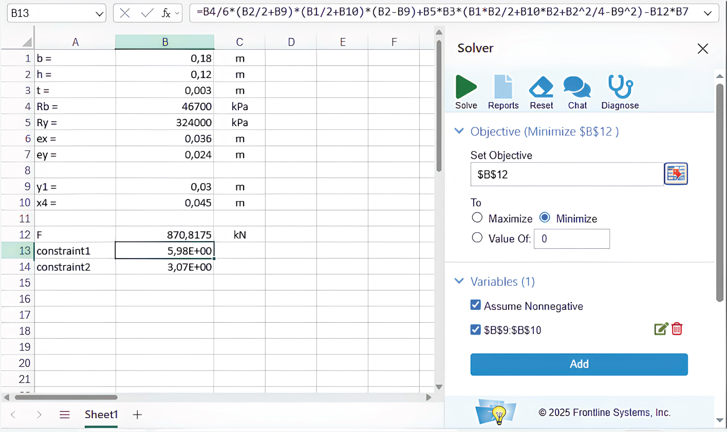
Next, we proceed to option 2, the destruction option. Determining the ultimate load according to this option, in addition to the Optimization Toolbox package of the MATLAB environment, is also available from Microsoft Excel when using the Solver add-in.
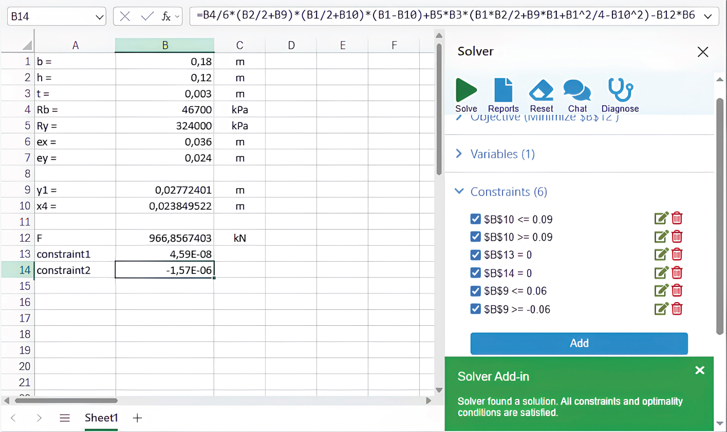
Fig. (10) shows a screenshot from the Microsoft Excel Online program. Cells B1:B7 represent the initial data. Cells B9:B10 are intended for the variables y1x4. The coordinates of the initial search point are entered into these cells, which we take to be equal to [h/4;b/4]. Cell B12 represents the objective function, which is determined by Eq. (23). Constraints “constraint1” and “constraint2” are determined based on Eqs. (26, 27). Fig. (11) illustrates all the constraints for this optimization problem, as well as the solution found. The solution was found, and all constraints were satisfied. The ultimate load according to option 2 was 967 kN, and the parameters y1 and x4, which determine the position of the neutral line, were equal to 0.0277 and 0.0238 m, respectively.
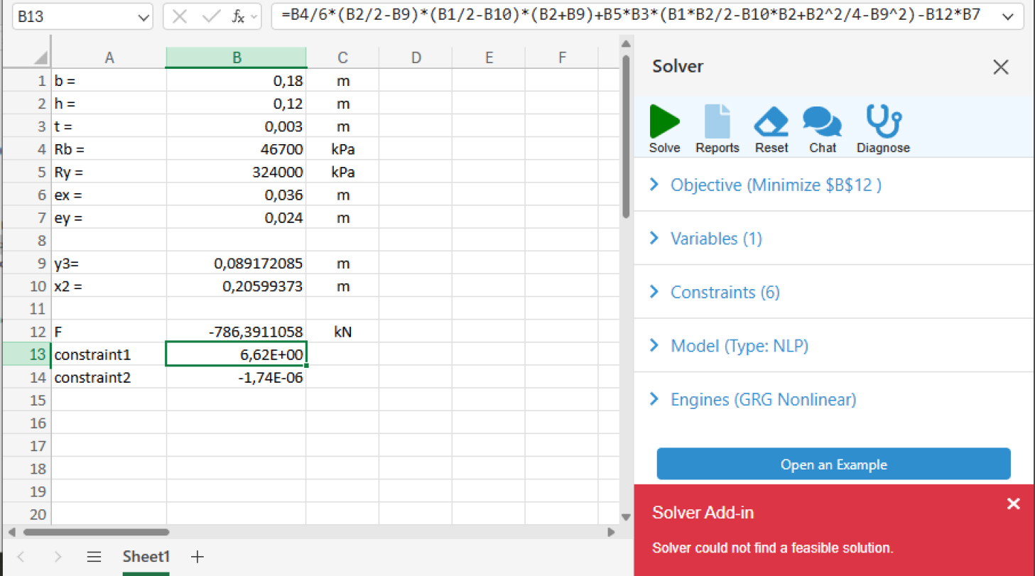
Let us now consider the destruction option 4. The solution is performed similarly to option 2. For this variant, the solver was unable to find a possible solution (Fig. 12), which indicates the impossibility of destruction according to option 4.
Thus, finally, according to the calculation results, destruction occurs according to option 2 at the ultimate load of Fult = 967 kN. The experimental value of the ultimate load is 939 kN, which differs by 2.9% from the theoretical value.
Screenshot from the Microsoft Excel Online program.
Constraints in the optimization problem and the result of finding a solution.
Result of searching for a solution for destruction according to option 4.
CONCLUSION
An analytical model is proposed for determining the bearing capacity of eccentrically compressed rectangular CFST columns in the presence of axial force eccentricities in two planes. The developed model is based on the limit equilibrium method. All possible variants of the compressed zone location in the cross section are considered, and for the considered variants, resolving equations are obtained that allow determining the ultimate load. For two possible failure schemes, the problem is reduced to a quadratic equation related to the ultimate load. For the other two schemes, the calculation is simplified to solving a system of three nonlinear equations, which can be performed using a publicly available tool such as Microsoft Excel Online.
The calculation method was tested on the results of experiments for 38 samples presented in three different works. The average value of the experimental ultimate load to the calculated ultimate load ratio is close to one, and the correlation coefficient between the experimental and calculated values of the ultimate load was 0.979. The calculation results obtained using the proposed analytical model are also very close to those of the finite element analysis. This suggests the potential application of the proposed model in engineering practice for preliminary bearing capacity assessments of rectangular CFST columns. To facilitate the reproduction of the results and their application in engineering practice, a numerical example of the calculation was also provided.
STUDY LIMITATIONS
The limitations of the model include that it does not take into account additional eccentricities of the axial force caused by the deflection of the element. The model is applicable for short columns whose slenderness ratio (the ratio of the calculated length to the minimum radius of gyration for reduced cross-section) does not exceed 14. Additionally, the proposed model overlooks the effects of local stability loss in the pipe wall, the work of the tensile zone in concrete, and the increase in the bearing capacity of the concrete core resulting from lateral compression. The confinement effect can be taken into account by adjusting the design strength of the concrete and steel pipe. Considering the effect of concrete lateral compression by the steel tube in the proposed model is a prospect for our further research.
AUTHORS’ CONTRIBUTIONS
The authors confirm their contribution to the paper as follows: A.C.: Study conception and design; V.T.: Analysis and interpretation of results; S.A.Z.: Draft manuscript. All authors reviewed the results and approved the final version of the manuscript.
LIST OF ABBREVIATIONS
| Rb | = Compressive strength of concrete |
| Ry | = Yield strength of the steel |
| b | = Cross-section width |
| h | = Cross-section height |
| ex, ey | = Axial force eccentricities along the x and y axes |
| t | = Thickness of the rectangular steel profile pipe |
| x2, x4, y1, y3 | = Distances determining the position of the neutral line |
| F | = Compressive force |
| Nb | = Axial compressive force perceived by concrete |
| Ns | = Axial compressive force perceived by steel |
| Mbx, Mby | = The concrete perceives bending moments in the x and y axes |
| Msx, Msy | = Bending moments in the x and y axes perceived by steel |
| Mx, My | = Total bending moments in the x and y axes |
| Nexp | = Experimental values of the ultimate load |
| Ncalc | = Analytical values of the ultimate load |
| NFEM | = Ultimate load values calculated by the finite element method |
AVAILABILITY OF DATA AND MATERIALS
The data and supportive information are available within the article.
ACKNOWLEDGEMENTS
Declared none.