All published articles of this journal are available on ScienceDirect.

Developing the Learning Curve Model to Enhance Construction Project Scheduling and Cost Estimating
Abstract
Aim
The aim of the study is to develop a scheduling and cost estimation model for repetitive construction units by applying the learning curve theory and to contribute to advancements in construction project management practices, promoting efficiency and competitiveness within the industry.
Background
Construction projects, particularly those with repetitive units like housing developments, face ongoing challenges in accurate scheduling and cost estimation. Traditional estimation methods often overlook the impact of learning effects, which can improve productivity and reduce costs as crews gain experience. Learning curve theory, widely applied in manufacturing, offers a framework to model these gains in construction settings. Integrating learning curves into project planning has the potential to enhance accuracy in forecasting timelines and budgets, ultimately improving project efficiency and resource management.
Objective
The objective of this study is to develop and apply a learning curve model to enhance scheduling and cost estimation in repetitive construction projects, particularly in a multi-unit housing project.
Methods
By incorporating historical data and analyzing critical factors that impact project duration and cost, a more reliable forecasting model is developed. The learning curves are created using a three-point approach, supported by artificial neural networks (ANN) and the relative importance index (RII), to systematically assess cost divisions and influential project factors.
Results
The results indicate that the learning curve model can achieve time savings of 27% and labor cost savings of 36% compared to traditional estimation methods that do not consider the effect of the learning curve in construction projects.
Conclusion
This research demonstrates that learning curve models, combined with advanced data analysis techniques, provide a robust framework for optimizing project schedules and budgets, ultimately leading to more efficient resource utilization and cost-effective project outcomes. In other words, the study presented in this paper is significant as it can lead to improved project outcomes, cost savings, better resource management, and overall advancement in the construction industry's practices and competitiveness. This approach allows for accurate scheduling and cost forecasting based on data-driven insights.
1. INTRODUCTION
The engineering and construction industry is essential to societies and economies worldwide, employing over 100 million people. Construction-related spending alone contributes approximately 13% to the global gross domestic product (GDP) [1]. Developing a schedule for construction projects is a big challenge for a schedular team, who try to achieve the high accuracy of the final schedule. However, collecting reliable data about the nature of the project’s activities can help to estimate the required time and cost of these activities and accordingly identify the project cost and schedule [2]. The required data to develop a project schedule includes but is not limited to several factors such as the available resources, geotechnical information, forecasting, efficiencies of the equipment, tools, tools technology, etc. These factors can be analyzed systematically to attain the activities input with one exceptional factor, which is the ability of the crew individually and in groups to perform these activities. In construction project management, accurate scheduling and cost estimation are crucial for successful project execution, especially for projects involving repetitive units, such as housing developments. A precise schedule and budget not only improve project feasibility but also enhance resource allocation and efficiency, reducing delays and cost overruns. However, developing reliable schedules and cost estimates remains a significant challenge due to the complexity and variability of construction activities. One method to address this complexity is by applying learning curve principles, which recognize that efficiency tends to improve with repetition. As tasks are repeated, teams gain experience, leading to shorter task durations and lower costs. Historical data can be combined with learning curve models to predict these efficiencies, providing a more accurate forecast for project timelines and budgets.
2. LITERATURE REVIEW
The learning curve is an important measure for evaluating human performance in perceptual learning. It can reflect several processes, such as overall learning, forgetting or consolidation between sessions, and rapid relearning, adaptation, or decline within a single session [3]. Findings from a study identified learning curve theory as it is based on the concept that productivity increases as tasks are repeated [2]. Meanwhile, it was noted in another related study that learning curves in the analysis of construction operations are considered a key factor in determining variations in on-site productivity and are consistently accounted for during the planning and estimation phases [4]. However, the time and effort required to complete repetitive tasks decreases as the number of repetitions grows, which can be attributed to several factors [5]. This includes greater worker familiarization, enhanced coordination between equipment and crews, improved job organization, stronger engineering support, better day-to-day management and supervision, development of more efficient techniques and methods, more effective material supply systems, and a stabilized design, resulting in fewer modifications and rework. However, learning curve theory is applied based on three conditions: repetitious, continuous, and essentially identical. Remarkably, many repetitive construction field operations follow a learning curve, where the time or cost per cycle reduces as the number of cycles increases [6]. Thus, it was identified that a learning curve is formed when the time or cost to complete a single cycle of an activity is plotted against the cycle number [7]. Essentially, for construction engineers and managers, the primary value of learning curves lies in their ability to forecast future performance, rather than just analyzing historical data. Mathematical learning curve models can predict the time or cost for future cycles in repetitive construction activities. Analysts can choose from various methods to represent the data, often balancing between the responsiveness and stability of the forecasting information [8]. It is emphasized that five models of learning curves, which are the straight-line power, the Stanford “B”, the cubic power, the piecewise, and the exponential [5]. The applications of the learning curve in the construction industry have been studied by several scholars, with most of these applications focusing on project cost, time, and performance. In addition, these studies pose a crucial question: which learning curve model is best suited to predict the future performance of a repetitive activity? A previous study forecasted the construction project costs using the learning curve with respect to Wright’s models and the one-factor learning curve model [9]. Similarly, a comparative analysis of learning curve models for the productivity of diaphragm wall and pile, according to six learning curve models, was performed [10]. Ultimately, it was concluded that the combined exponential log-linear model is the most suitable fit for both applications. As pointed out earlier, five learning curve models were compared using unit and cumulative productivity data based on historical data from the construction of thirty-four caissons fabricated with the slip form technique over an eight-month period [4]. The authors applied a linear model to assess the learning curve effect in high-rise floor construction [11]. Likewise, a research was conducted to link the crew skill coefficient to the learning curve of a specific repetitive task [12]. Moreover, a study examined the impact of repeated building floor layouts on formwork labor productivity [13] while, an analysis was carried out to determine the factors affecting the manifestation process to propose a more appropriate learning curve model for high-rise construction activities such as task variation and work adaptation [14].
Table 1 shows previous studies focusing on selecting the best learning curve model or method for predicting future productivity. From the table, it is obvious that there is hardly any model that effectively addresses repetitive construction activities, particularly when forecasting productivity for different construction projects. Furthermore, most of these studies concentrate on specific construction activities without accounting for the interconnected nature of various divisions within a project,
| Learning Curve Model/method | Best Fit | Repetitive Construction Activity | Refs. |
|---|---|---|---|
| Stanford “B,” piecewise, straight-line, cubic, and exponential | • The cubic model | • Precast Floor Planks | [5] |
| Linear x, y; linear, x, log y; linear log x, y; linear log x, log y; quadratic x, y; quadratic x, log y; quadratic log x, y; quadratic log x, log y; cubic x, y; cubic x, log y; cubic log x, y; and cubic log x, log y | • The cubic model for the available historical data only • Linear models for future predictions |
• 60 different construction activities | [6] |
| Unit data, cumulative-average data, moving average, and exponentially weighted average | • Unit data | • 60 different construction activities | [8] |
| Three-parameter hyperbolic, Two-parameter hyperbolic, Three-parameter exponential, Two-parameter exponential, and Log-linear | • The three-parameter hyperbolic | • Contractor performance | [15] |
| Straight Line, Quadratic, Cubic, Combined Exponential Log-linear, and Stanford B | • Combined Exponential Log-linear | • Diaphragm wall and pile | [10] |
| Stanford “B,” piecewise, straight-line, cubic, and exponential | • Cubic model fits historical data • Stanford “B” model provides better future predictions |
• Caisson fabrication process | [4] |
which can influence the overall project duration and cost. Additionally, the learning curves developed in these studies rely on available data, which is often challenging to obtain during the early stages of a construction project. In addition, to address this gap, the current research introduces a comprehensive model that utilizes limited data from the early stages to estimate project duration and forecast project costs.
3. METHOD
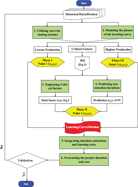
Fig. (1) illustrates the development of the learning curve for the cost division. The six steps (highlighted in green) for developing the learning curve model are as follows: utilizing cost-estimating systems, modeling the phases of the learning curve, employing critical factors, predicting construction duration, integrating duration estimation with learning rates, and forecasting project duration and cost. These steps are detailed in subsections 3.1 through 3.6.
3.1. Utilizing Cost-estimating Systems
Cost estimating systems help identify the various divisions and activities within a construction project. Systems such as Uniformat, Master, or others can be selected based on the specific needs of the research. For this study, the uniformat cost estimating system [16], which organizes the project into 12 divisions, was chosen for its simplicity and applicability. Each division is examined to determine whether it involves repetitive activities. For example, division 10 (general conditions & profit) does not contain repetitive tasks, and therefore, the learning curve is not applied to this division.
3.2. Modeling the Phases of the Learning Curve
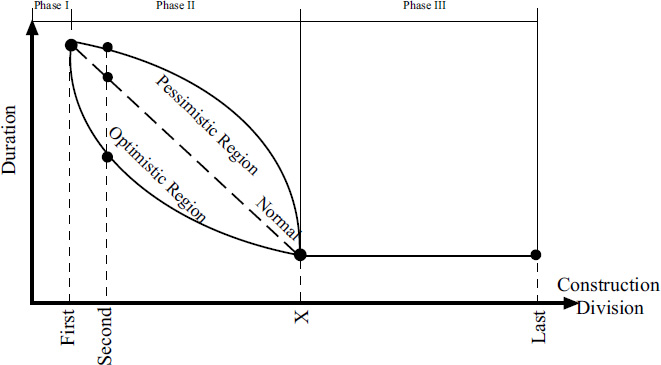
Figs. (2 and 3) illustrates the developed learning curve structure based on the duration required to complete similar units in a cost division in construction. This curve is divided into three key phases: (a) the learning phase (Phase I), (b) the acceleration phase (Phase II), and (c) steady-state phase (Phase III). Phase I marks the beginning of work on an activity where the crew requires the maximum time to complete a unit compared to future units performed by the same team. In Phase II, the crew progressively needs less time to complete similar units, thanks to factors such as improved efficiency and familiarity. However, the rate of acceleration can vary; it may be slow, normal, or rapid. Furthermore, by analyzing the influence of specific factors on crew productivity, the acceleration rate can be positioned within a pessimistic range (for a lower rate) or an optimistic range (for a higher-than-normal rate). Additionally, to better predict this phase, a model is needed to connect these factors to productivity rates, thus shaping the learning curve during planning. Phase III represents the minimum time required by the crew to complete each unit, beyond which no additional time savings are achievable. Consequently, the curve in this phase becomes consistent, reflecting a steady state. Moreover, to accurately forecast the necessary duration and cost, it is essential to incorporate realistic assumptions and account for variations in crew performance and external conditions.
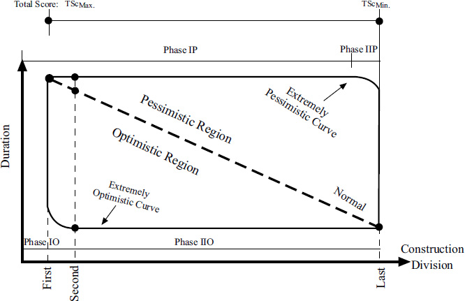
In addition,to derive the learning curve for a specific construction division, it is assumed that the curve may reach extreme outcomes under optimistic and pessimistic scenarios. This assumption is made to account for all possible scenarios that may arise during construction. In both cases, the learning curve is simplified into two phases rather than three. Under the optimistic scenario, where learning is rapid, the curve progresses directly to the second phase (IIO) following the completion of the first unit. Conversely, in the pessimistic scenario, a significant amount of time is required to transition into the second phase (IIP), reflecting a slower rate of improvement. Moreover, to forecast the duration of a division based on the learning curve, three key points are needed to define the curve. The first point marks the beginning, where the time required to complete an activity is at its maximum. The second point is an intermediate value on the curve, located between the first and last points. The third point represents the end of the curve, where the required duration reaches its minimum. Historical data is invaluable in identifying the first and third points by considering the critical factors outlined in the next section. These factors have a direct impact on predicting the duration of the new project, as summarized in Table 2.
Project methodology.
| Point | First Point (x1,y1) |
Second Point (x2,y2) | Third Point (x3,y3) |
|---|---|---|---|
| Duration | Maximum | Between | Minimum |
| Case | Extreme Pessimistic | Between | Extreme Optimistic |
| Critical Value (Total Score-TSc) |
Minimum | Between | Maximum |
Learning curve structure.
The developed learning curve structure.
Using historical data, it identifies the lowest and highest productivity levels along with the critical factors influencing manpower productivity in each project division. The developed curve comprises three key points:
1. Point (x1, y1): Represents the lowest productivity.
2. Point (x2, y2): Determined through the total score (TSc) and prediction process, which will be discussed in sections 3.3 and 3.4.
3. Point (x3, y3): Represents the highest productivity.
It should be noted that xi represents the ith unit. For example, if a project includes 30 units, i ranges from 1 to 30. Similarly, yi denotes the required duration (in days) to complete the ith unit.
3.3. Employing Critical Factors
The optimistic and pessimistic learning curves are directly influenced by various factors that impact the rate of learning. Moreover, to understand and accurately forecast this rate, it is essential to study, prioritize, and select the most significant factors. Table 3 lists 21 critical factors [17-22] that have been identified as affecting the learning rate of repetitive activities division, with their effects varying depending on the type of division. Analyzing these impacts is crucial for developing the mathematical model of the learning rate, as explained in the following section. The set of 21 factors can be expanded or narrowed based on the specific needs and nature of the construction project.
| No. | Factor |
|---|---|
| CF1 | Worker Competence |
| CF2 | Experience |
| CF3 | Weather Conditions |
| CF4 | Site Conditions |
| CF5 | Accessibility |
| CF6 | Availability of tools and Equipment |
| CF7 | Quality and Maintenance of tools and Equipment |
| CF8 | Supply Chain Efficiency of Materials |
| CF9 | Quality of Materials |
| CF10 | Planning and Scheduling |
| CF11 | Coordination and Communication |
| CF12 | Leadership |
| CF13 | Wages and Incentives |
| CF14 | Work Hours |
| CF15 | Safety Measures |
| CF16 | Worker Health |
| CF17 | Automation and Digital Tools |
| CF18 | Team Dynamics |
| CF19 | Worker Satisfaction |
| CF20 | Regulatory Requirements |
| CF21 | Economic Conditions |
In this research, the top five factors are selected using the relative importance index (RII) method. However, a decision-maker looking to adopt this research can freely adjust the selected factors, increasing or decreasing them to suit the specific circumstances of a new project. From a personal perspective, including too many factors can make calculations unnecessarily complex. RII is a statistical tool widely used in construction research to rank factors based on their relative significance. It is calculated by normalizing the responses of survey participants to ensure comparability. RII is expressed as a value between 0 and 1, with higher values indicating greater importance. This method is particularly useful for prioritizing critical factors affecting construction projects, such as delays, costs, or risks. Furthermore, by identifying the most significant elements through RII, decision-makers can focus on key areas for improvement or resource allocation [23]. RII requires conducting a questionnaire survey to obtain factor values, which are then used to rank these factors by importance. Additional factors can be included in the analysis if the decision-maker chooses to expand the scope. The formula for calculating the RII is provided in Eq. (1).
 |
(1) |
Where A = ∑a, and n = 1,2,... ., N. In this context, “A” denotes the total number of responses, while “n” represents the scale of importance assigned to each factor, ranging from “1” up to “N”. After identifying the top five factors, the total score (TSc) for each construction division can then be calculated using Eq. (2).
| TSci = ∏ CFi | (2) |
The scale for each critical factor (CF) ranges from 1 to 4, with “1” indicating a very low value and “4” indicating a very high value. Consequently, the TSc for each division extends from TScMin. to TScMax., assuming the critical factors are independent of each other. For example, in an optimal scenario where factors like weather, experience, site conditions, tool availability, and wages are each assigned a score of 4, the resulting total score would be (TSc=45=1024). Conversely, in the most pessimistic case, where all critical factors are rated at the minimum, the TSc value for the division would be 1, while a score of 45 (or 1024) would indicate the most favorable conditions, as illustrated in the previous example. For a new project, data on these factors should be collected from both past and current projects. In this study, only the top five factors will be considered, as discussed.
3.4. Predicting Construction Duration
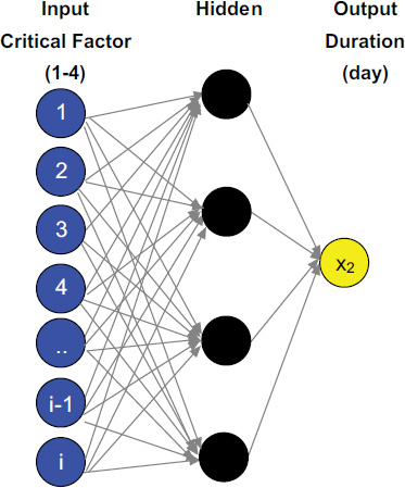
Based on historical data, the first point (x1=1, y1=DurationMax.) represents the initial construction unit of the specific division, characterized by the maximum duration. The second point (x2,y2) corresponds to the coordinates of the new project currently under study. The third point (x3=last unit, y3 = DurationMin.) marks the final construction unit in the division, associated with the minimum duration. The first coordinate (x2) can be determined using Eq. (2), considering the levels of critical factors that influence the learning rate. The TSc value of the new project represents (x2). Additionally, to estimate the value of y2, predictions can be generated using an artificial neural network (ANN) tool, as illustrated in Fig. (4).
ANN model for the duration of the construction division.
The Artificial Neural Network (ANN) method was selected to predict the division durations due to its ability to model complex, non-linear relationships and learn from historical data. This approach offers flexibility in handling diverse input factors, making it well-suited for predicting durations across various construction divisions. Additionally, ANN models can improve prediction accuracy as they adapt and learn from new data, providing more reliable forecasts for project scheduling and cost estimation.
Using the critical factors' scale of 1 to 4, the duration (y2) for the new project can be predicted. However, a substantial amount of data is needed to effectively train and test the network to achieve high prediction accuracy and minimize errors. NeuralTools 7.5 [24] streamlines the process of implementing neural networks for predictive analytics, making it an excellent choice for professionals in fields like engineering, finance, and project management. While it has limitations in terms of data dependency and interpretability, its user-friendly design and integration with Excel make it a valuable tool for tackling both classification and regression problems. By following the outlined process, users can effectively leverage NeuralTools to gain actionable insights and improve decision-making in their projects. The structure of the developed ANN model for determining the division duration (y2) consists of three layers: input, hidden, and output. The input layer includes the critical factors affecting the construction project, as outlined in Table 3. The model requires data input from several construction projects, including their associated critical factors and corresponding durations. For this research, the input layer incorporates data from multiple projects, with each project defined by its critical factors. These factors may include all or a subset of the listed factors, depending on the specific characteristics of the project. It is essential to rank these factors and select those with the highest relevance to ensure the prediction model’s accuracy and efficiency. For instance, if the input layer represents ten projects and the top critical factors selected are five, the input layer will comprise 50 nodes. Each node is assigned a value on a scale of 1 to 4, where “1” represents a very low impact and “4” indicates a very high impact on the learning curve’s performance. The number of nodes in the hidden layer is automatically determined by NeuralTools 7.5 [24] without user intervention. However, if users wish to manually control the number of nodes in the hidden layer, NeuralTools 7.5 may not be the ideal tool for such customization. The output layer produces the predicted duration for the new project based on its associated critical factors.
With this second point established, the learning curve for each construction unit within each division can then be developed.
3.5. Integrating Duration Estimation and Learning Rates
Determining the duration of all construction units within each division is essential for first developing the project schedule and then estimating its cost for each cycle. This serves as the foundation for the subsequent cycle, considering the learning rates of the next phase. Additionally, the logical relationships among divisions, including the lag and lead times, remain consistent across all cycles.
3.6. Forecasting the Project Duration and Cost
After completing the scheduling and cost estimation for each cycle, the final step involves updating the learning curves for each division of the project. With each cycle, new data is incorporated into the learning curve, continuing until all cycles, which represent the construction units of every division, are completed. The finalized learning curves for all divisions can then be used to predict the future schedule and cost of the repetitive construction project units. Once this scheduling is completed, the project's cost estimates can be derived based on the identified activities [25].
Validation of the scheduling and cost estimation process is crucial for updating the learning curve and ensuring its applicability in subsequent cycles. For each cycle, it is necessary to evaluate whether external or internal factors have influenced the behavior of the developed learning curve. If no changes are detected, the existing learning curve can be directly applied to the next cycle. However, if changes are identified, the model must
| Division | P2* | P3* | P4* | P5* | P6* | P7* | P8* | P9* | P10* | P11* | Point 1 (1, Max.) | Point 3 (30, Min.) |
|---|---|---|---|---|---|---|---|---|---|---|---|---|
| Foundation | 30 | 35 | 36 | 28 | 34 | 29 | 37 | 37 | 40 | 40 | (1,40) | (30,28) |
| Substructure | 25 | 31 | 25 | 24 | 27 | 23 | 28 | 26 | 30 | 32 | (1,32) | (30,23) |
| Superstructure | 60 | 77 | 67 | 60 | 61 | 61 | 75 | 64 | 76 | 76 | (1,77) | (30,60) |
| Exterior Closure | 43 | 52 | 47 | 44 | 46 | 42 | 53 | 50 | 52 | 54 | (1,54) | (30,42) |
| Roofing | 6 | 10 | 5 | 8 | 6 | 6 | 8 | 7 | 11 | 12 | (1,12) | (30,5) |
| Interior Construction | 17 | 31 | 18 | 20 | 19 | 17 | 29 | 27 | 32 | 31 | (1,32) | (30,17) |
| Mechanical | 16 | 26 | 20 | 18 | 19 | 17 | 24 | 24 | 26 | 26 | (1,26) | (30,16) |
| Electrical | 15 | 26 | 21 | 14 | 16 | 15 | 24 | 23 | 25 | 24 | (1,26) | (30,14) |
| Site Work | 23 | 21 | 23 | 24 | 22 | 20 | 31 | 30 | 31 | 32 | (1,32) | (30,20) |
| No. | Critical Factor | 1 | 2 | 3 | 4 | 5 | Total | RII |
|---|---|---|---|---|---|---|---|---|
| 1 | Experience | 5 | 5 | 10 | 41 | 78 | 139 | 0.862 |
| 2 | Wages and Incentives | 8 | 11 | 21 | 44 | 55 | 139 | 0.783 |
| 3 | Availability of tools and Equipment | 12 | 23 | 35 | 36 | 33 | 139 | 0.679 |
| 4 | Site Conditions | 15 | 12 | 46 | 37 | 29 | 139 | 0.676 |
| 5 | Weather Conditions | 12 | 31 | 30 | 28 | 38 | 139 | 0.671 |
be revised to incorporate these modifications (this refinement is beyond the scope of the current paper). This iterative approach continues until all construction units are completed, at which point the learning curve reaches its final, stable form. To validate the current research, the planning team of the company responsible for constructing the 30-unit housing project conducted a SWOT analysis to evaluate the strengths, weaknesses, opportunities, and threats associated with the developed models.
4. RESULTS
To apply the developed learning curve model to a construction project division, a 30-unit housing project is selected. This project is being executed by a Saudi construction company that utilizes its own resources for design and construction, with the goal of investment. The company has engaged subcontractors for each of the 9 cost estimating divisions to perform the necessary activities. Note that division 10 (general conditions and profit) is excluded as it is managed by the owner. Division 7 (conveying systems) is also omitted, as it is not applicable to this unit. Additionally, division 11 (equipment) has been merged with division 8 (mechanical) due to its limited scope. Crew groups are assigned to similar tasks across the 30-unit project. Given the repetitive nature of these activities, the learning curve principle is employed to assist in scheduling and cost estimation. Historical data from 10 previous projects has been collected to implement the model, as shown in Table 4. The square meter method is utilized to adjust the durations of previous projects, making them comparable to the new project. It is important to note that P1 is designated for the new project. For the new project's nature, which involves a one-floor housing design, division 11 (equipment) is combined with division 8 (mechanical), while division 7 (conveying systems) is excluded. Based on historical data, points 1 and 3 of the learning curve for each division are determined. For example, for the foundation division, point 1 and point 3 are determined as x1=1 for the first unit and x3=30 for the last unit. The corresponding durations are y1=40, based on projects 10 or 11, which had the maximum duration, and y3=28, based on project 5, which had the minimum duration among the other projects.
The next step is to determine the second point (x2,y2) of the learning curves for the construction divisions. First, the top critical factors are identified using Table 3 and Eq. (1). A questionnaire survey is conducted with 139 specialists in construction management to assign a level of importance, ranging from 1 to 4, to each critical factor. Accordingly, using Eq. (1), the experience factor is calculated as follows:
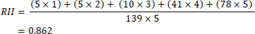 |
Similarly, the RII of other factors is calculated and presented in Table 5. The table highlights the top five factors in order: Experience, Wages and Incentives, Availability of Tools and Equipment, Site Conditions, and Weather Conditions. Other critical factors, which are not listed in Table 5, were also considered but ranked lower. The top five factors were selected by the planning department manager based on their simplicity and data availability. Including additional factors could complicate the process and make data collection more challenging.
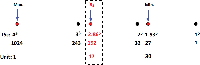
Using Eq. (2) and the level of the new project, the TSc for each project was determined, as shown in Table 6. TScmin=27 and TScmax=1024, while the TSc for the new project is 192.
Fig. (5) illustrates the linear interpolation used to determine the value of x2, which is found to be 17. This value is consistent across all construction divisions of the project since they pertain to the same overall project scope. The interpolation calculations are as follows:
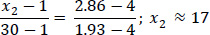 |
The final step is to determine the value of y2 (the duration for each division), which varies for each division. Using NeuralTools 7.5 [24], the predicted duration for the first division (foundation) of the new project is 34 days, as shown in Table 7. The input data includes the levels of critical factors (rated 1–4) and the durations (in days) for the specific division across the previous ten projects (P2–P11), which are used for training and testing. For the new project (P1), only the levels of the critical factors are included.
The dataset of ten projects was split into 80% for training and 20% for testing using NeuralTool 7.5 to predict the durations of the divisions. A summary of the output report generated using NeuralTool 7.5 (Table 8) shows that the developed model consists of a generalized regression neural network (GRNN) for all divisions. The number of trials varies among the divisions, and the percentages of bad predictions and root mean square error are very low, indicating that the results are acceptable.
| Project | Experience | Wages and Incentives | Availability of Tools and Equipment | Site Conditions | Weather Conditions | TSci (Eq. 2) |
|---|---|---|---|---|---|---|
| P1 | 4 | 3 | 4 | 2 | 2 | 192 (New Project) |
| P2 | 3 | 3 | 4 | 4 | 4 | 576 |
| P3 | 3 | 2 | 3 | 3 | 3 | 162 |
| P4 | 4 | 3 | 4 | 4 | 2 | 384 |
| P5 | 4 | 3 | 4 | 3 | 4 | 576 |
| P6 | 3 | 4 | 3 | 4 | 4 | 576 |
| P7 | 4 | 4 | 4 | 4 | 4 | 1024 (TScmax.) |
| P8 | 2 | 3 | 4 | 3 | 3 | 216 |
| P9 | 4 | 4 | 3 | 3 | 3 | 432 |
| P10 | 2 | 2 | 3 | 3 | 1 | 36 |
| P11 | 3 | 1 | 3 | 3 | 1 | 27 (TScmin.) |
x2 value using linear interpolation.
| Oject | Experience | Wages and Incentives | Availability of Tools and Equipment | Site Conditions | Weather Conditions | Duration | Tag Used | Prediction | Good/Bad | Residual |
|---|---|---|---|---|---|---|---|---|---|---|
| P1 | 4 | 3 | 4 | 2 | 2 | 34 | predict | 34 | - | - |
| P7 | 4 | 4 | 4 | 4 | 4 | 28 | train | - | - | - |
| P2 | 3 | 3 | 4 | 4 | 4 | 29 | train | - | - | - |
| P5 | 4 | 3 | 4 | 3 | 4 | 31 | test | 29 | Good | 2 |
| P6 | 3 | 4 | 3 | 4 | 4 | 33 | train | - | - | - |
| P4 | 4 | 3 | 4 | 4 | 2 | 30 | train | - | - | - |
| P9 | 4 | 4 | 3 | 3 | 3 | 34 | train | - | - | - |
| P8 | 2 | 3 | 4 | 3 | 3 | 39 | train | - | - | - |
| P3 | 3 | 2 | 3 | 3 | 3 | 37 | train | - | - | - |
| P10 | 2 | 2 | 3 | 3 | 1 | 39 | test | 40 | Good | -1 |
| P11 | 3 | 1 | 3 | 3 | 1 | 40 | train | - | - | - |
| Division | Configuration | Training | Testing | |||
|---|---|---|---|---|---|---|
| Number of Trials | % Bad Predictions (30% Tolerance) | Root Mean Square Error | % Bad Predictions (30% Tolerance) | Root Mean Square Error | ||
| Foundation | GRNN Numeric Predictor | 146 | 0.00 | 0.00135933 | 0.00 | 1.863536141 |
| Substructure | GRNN Numeric Predictor | 116 | 0.00 | 0.0000000 | 0.00 | 2.474873734 |
| Superstructure | GRNN Numeric Predictor | 113 | 0.00 | 0.64030543 | 0.00 | 1.275221115 |
| Exterior Closure | GRNN Numeric Predictor | 108 | 0.00 | 0.536803405 | 0.00 | 1.178468891 |
| Roofing | GRNN Numeric Predictor | 95 | 0.00 | 0.447752892 | 0.00 | 0.71351039 |
| Interior Construction | GRNN Numeric Predictor | 160 | 0.00 | 0.143800477 | 0.00 | 2.384358823 |
| Mechanical | GRNN Numeric Predictor | 56 | 0.00 | 0 | 0.00 | 1.986281073 |
| Electrical | GRNN Numeric Predictor | 55 | 0.00 | 0 | 0.00 | 3.482097069 |
| Site Work | GRNN Numeric Predictor | 78 | 0.00 | 0.294408522 | 0.00 | 1.027706774 |
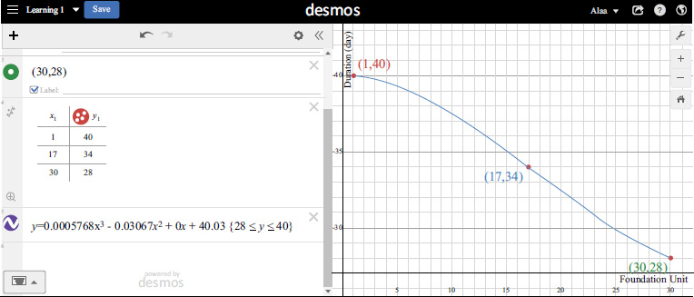
Foundation learning curve using desmos.
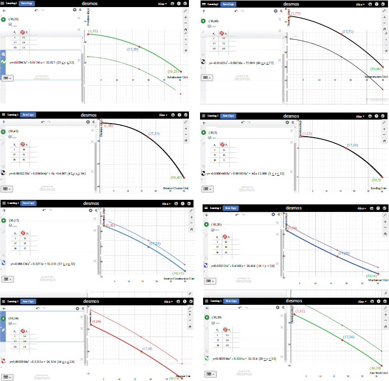
Learning curves for the 30 house-units according to the construction divisions using desmos.
With (x2,y2) identified, the learning curve for the foundation division is generated using the online tool, which is called Desmos [26], as shown in Fig. (6). The foundation curve is positioned in the optimistic region, with its equation displayed in the figure. Additionally, the duration for the foundation division across all 30 units can be calculated using this learning curve. Similarly, learning curves for the remaining divisions are developed (Fig. 7), allowing for the overall schedule and cost estimate to be determined.
The summary of the properties of the developed learning curves for the project's divisions is presented in Table 9. The best-fit curves are either quadratic or cubic, with an R-squared value equal to one. Most developed learning curves fall within the pessimistic range, indicating slower-than-normal crew productivity, except for the foundation and mechanical divisions, which are in the optimistic range. The learning curves span a domain of 1 to 30, based on the project's 30 housing units, while the ranges vary across divisions due to differences in their respective durations.
| Div.# | Division | Regression Type | Learning Curve Equation | Region | Domain | Range |
|---|---|---|---|---|---|---|
| 1 | Foundation | Cubic | y=0.0005768x3-0.03067x2+40.03 | Optimistic | 1-30 | 28-40 |
| 2 | Substructure | Quadratic | y=-0.00945x2-0.01741x+32.027 | Pessimistic | 1-30 | 23-32 |
| 3 | Superstructure | Quadratic | y=-0.01625x2-0.08256x+77.099 | Pessimistic | 1-30 | 60-77 |
| 4 | Exterior Closure | Cubic | y=0.0002259x3-0.006564x2+54.007 | Pessimistic | 1-30 | 42-54 |
| 5 | Roofing | Cubic | y=-0.00006488x3-0.005838x2+12.006 | Pessimistic | 1-30 | 5-12 |
| 6 | Interior Construction | Quadratic | y=-0.006134x2-0.3271x+32.333 | Pessimistic | 1-30 | 17-32 |
| 8 | Mechanical | Quadratic | y=0.002321x2-0.4168x+26.414 | Optimistic | 1-30 | 16-26 |
| 9 | Electrical | Quadratic | y=-0.002984x2-0.3213x+26.324 | Pessimistic | 1-30 | 14-26 |
| 12 | Site Work | Quadratic | y=-0.002984x2-0.3213x+32.324 | Pessimistic | 1-30 | 20-32 |
The schedule for the first unit is shown in Fig. (8), with a maximum duration of 284 days. Identifying critical and non-critical divisions is essential to optimize resource allocation and prevent delays. In this context- division 5 (roofing), division 8 (mechanical) and division 9 (electrical) are non-critical allowing their respective crews some flexibility in performing these tasks. The labor cost estimate for the first housing unit is 175-000 SAR, based on a duration of 284 days. Moreover, by applying the impact of the learning rate based on the learning curves of the respective divisions, the duration and labor cost estimates for the remaining 29 units can be projected, as shown in Fig. (9). The duration and labor cost estimates of unit 30 are 207 days and 111-332 SAR respectively, which means that saving time and labor cost estimates reached 27% and 36% respectively.
5. DISCUSSION
The developed learning curves for the construction divisions are categorized into quadratic and cubic models, reflecting the unique characteristics of each division’s activities. Quadratic models are predominantly applied to divisions such as substructure, superstructure, interior construction, mechanical, electrical, and site work, where repetitive tasks are common, and learning curve effects are more straightforward to model. In contrast, the foundation, exterior closure, and roofing divisions exhibit more complex behaviors, necessitating cubic models that better capture variations in productivity trends. This categorization provides a tailored approach to modeling productivity and cost improvements across different construction activities. Compared to previous studies, as shown in Table 1, the majority of divisions align with quadratic models, confirming their suitability for repetitive activities. However, the use of cubic models for select divisions indicates the flexibility of the developed methodology to adapt to unique project dynamics. Furthermore, by considering both quadratic and cubic models, the research bridges a critical gap, offering a nuanced understanding of productivity patterns in construction projects.
Additionally, by applying curve principles, this study demonstrates notable improvements in measuring productivity over time. As crews gain experience and efficiency through repetitive tasks, the effects of the learning curve lead to substantial reductions in both project duration and labor costs. For example, divisions with high adaptability to learning curves show accelerated productivity, ultimately resulting in time and cost savings. These results highlight the practical benefits of incorporating learning curve principles into project planning. The findings illustrate how leveraging learning curves can optimize construction schedules and labor costs for repetitive activities, offering a systematic approach to forecasting and managing project performance. This approach not only improves efficiency and resource utilization but also allows stakeholders to make informed, data-driven decisions. Such insights are particularly relevant for large-scale housing projects, where repetitive tasks predominate, providing significant opportunities for strategic planning and cost management.
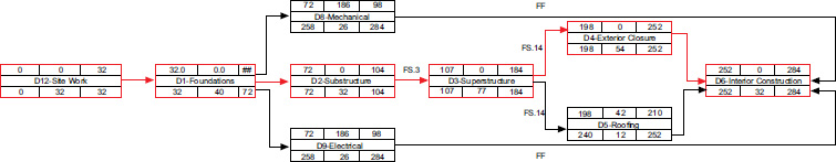
Project schedule of the first unit.
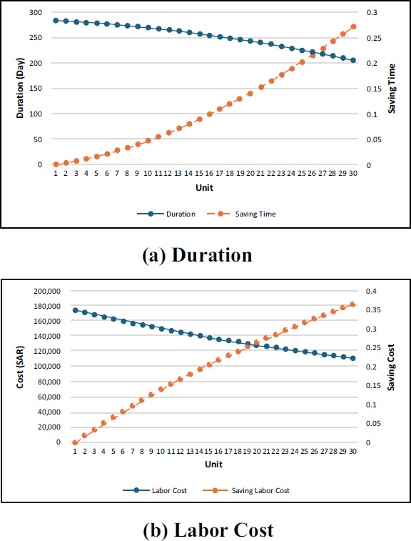
Project (a) duration and (b) labor cost for a 30 unit-housing project considering the impact of learning curve.
Moreover, by aligning learning curve models with project-specific needs, stakeholders can better anticipate challenges, allocate resources, and enhance overall project outcomes. The novelty of the current research, compared to previous studies, can be summarized as follows:
i. The developed learning curve integrates historical data from similar project types with critical factors affecting the project. This integration improves accuracy by adjusting historical data to align with the requirements of the new construction project during the planning stage.
ii. While the use of historical data is not new, this study emphasizes the adoption of such data within optimistic and pessimistic regions, providing a robust framework for evaluating potential variations in productivity.
iii. The learning curve methodology is applied comprehensively across all construction project divisions, enabling the development of an integrated schedule and accurate cost forecasts for the entire project. This holistic
| Strengths | Weaknesses |
|---|---|
| • High Applicability: The models demonstrate a very high level of relevance and usefulness across different projects. • High Adaptability: The models are highly adaptable, making them versatile for various construction scenarios. • Reliable Project Time and Cost Predictions: The models provide consistent and dependable results for estimating project time and costs. |
• Resource Sensitivity: The models are significantly affected by changes in resource availability, which could limit their accuracy. • Dependence on Critical Factors: Adjusting the total score of critical factors for unforeseen risks introduces a potential margin of error. |
| Opportunities | Threats |
| • Risk Management Integration: Refining the critical factor adjustment process to better account for unforeseen risks could improve the model’s resilience and accuracy. • Scalability: With further development, the models could be scaled to more complex projects, increasing their utility across larger construction initiatives. • Enhanced Forecasting Tools: Developing supplementary tools to anticipate resource changes can strengthen the reliability of outcomes. |
• Unpredictable Risks: Unexpected external factors (e.g., economic changes and supply chain disruptions) may impact the model’s effectiveness. • Over-Reliance on Input Data: The accuracy of the models heavily depends on the quality of input data, making them vulnerable to errors or incomplete datasets. • Dynamic Resource Environments: Projects in rapidly changing environments may struggle to fully benefit from the model without constant recalibration. |
approach accounts for interdependence between divisions, ensuring a more cohesive and reliable project plan.
iv. This approach introduces a new estimation tool for engineers, planners, and practitioners during the early stages of construction projects, where available data is often limited. By relying on limited but strategically utilized data, the model ensures practical applicability even in scenarios with constrained information.
In summary, this research advances the understanding of learning curve applications in construction projects. By tailoring models to division-specific needs and leveraging both historical data and critical factors, it sets a new benchmark for productivity analysis and cost forecasting in repetitive construction activities. These contributions not only validate the practicality of the methodology but also provide actionable insights for improving project performance across various construction domains.
6. VALIDATION
The findings have been validated by the planning department members of the company executing the 30 housing units, with feedback summarized in Table 10. The feedback received provides valuable insights into the performance, applicability, and adaptability of the developed models for construction project management. These models have been designed to estimate acquisition time, project cost, and duration while accounting for critical factors that influence construction outcomes. The assessment also identifies limitations and suggestions for improvement, particularly in addressing unforeseen risks and resource variability. By examining the strengths, weaknesses, opportunities, and threats (SWOT) associated with the feedback, this analysis highlights the models' overall effectiveness and areas for enhancement to better support construction project planning and execution.
7. LIMITATIONS
While this study demonstrates the potential of learning curve models for improving scheduling and cost estimation in repetitive-unit construction projects- several limitations should be acknowledged.
1) The accuracy of the learning curve model relies heavily on the availability and quality of historical data; projects without sufficient or reliable data may not achieve the same level of precision in estimates.
2) The model assumes consistent crew performance and similar working conditions across units which may not always hold true due to variations in labor efficiency unexpected site conditions or fluctuating resource availability.
3) The application of ANN and the RII also requires specialized expertise and computational resources which may be challenging for smaller firms or projects with limited budgets.
4) The learning curve model is primarily suited to projects with repetitive units and its applicability may be limited in complex or unique construction projects with high variability across tasks.
8. FUTURE WORK
Building on the findings of this study future work could focus on
1) expanding the application of learning curve models to a wider variety of construction project types including those with complex non repetitive activities. By exploring the adaptability of learning curve models in diverse project environments- researchers can assess the potential benefits and limitations of these models beyond repetitive-unit construction.
2) Investigating the integration of additional variables such as real-time weather data supply chain dynamics labor availability and unexpected site conditions to enhance model accuracy under varying circumstances. Incorporating these factors could lead to a more robust and adaptable model providing even greater accuracy in scheduling and cost estimation.
3) Working on machine learning such as deep learning algorithms could also be explored to improve the predictive capabilities of the ANN model potentially increasing its precision and scalability.
4) Examining the use of dynamic learning curves that adjust in real-time based on project progress and feedback allowing for adaptive scheduling and cost adjustments as the project advances.
5) Validating these models in field conditions across multiple projects would provide practical insights and help establish best practices for implementing learning curve strategies. This validation could guide construction managers in optimizing resource allocation improving project outcomes and making data-driven decisions more accessible across the industry.
CONCLUSION
The study successfully achieved its aim of developing a scheduling and cost estimation model for repetitive construction units by utilizing the learning curve theory. By integrating learning curve principles into project management practices, the research contributes significantly to the advancement of construction project management, fostering efficiency and competitiveness within the industry.
Construction projects, especially those involving repetitive units like housing developments, often encounter challenges related to accurate scheduling and cost estimation. The traditional methods frequently fail to consider the benefits of learning effects, which can enhance productivity and reduce costs as work crews accumulate experience. Leveraging learning curve theory, commonly applied in manufacturing, provides a valuable framework for modelling these improvements in construction settings. The integration of learning curves into project planning holds promise for enhancing the precision of timeline and budget forecasts, ultimately enhancing project efficiency and resource utilization.
Through the development and application of a learning curve model in repetitive construction projects, particularly in multi-unit housing projects, this study addressed the objective of improving scheduling and cost estimation accuracy. By analyzing historical data and identifying critical factors influencing project duration and cost, a more dependable forecasting model was established. The utilization of a three-point approach to creating learning curves, supported by artificial neural networks (ANN) and the relative importance index (RII), systematically evaluated cost divisions and influential project factors.
The results obtained from the study are significant, showcasing that the learning curve model can lead to substantial time savings of 27% and labor cost reductions of 36% compared to traditional estimation methods that do not account for the learning curve effect in construction projects. This outcome underscores the potential benefits of incorporating learning curve models into construction project management practices.
Finally, this research highlights the efficacy of learning curve models when combined with advanced data analysis techniques, offering a robust framework to optimize project schedules and budgets. By enhancing resource utilization and facilitating cost-effective project outcomes, this approach not only enables accurate scheduling and cost forecasting but also contributes to improved project outcomes, cost savings, better resource management, and overall advancements in construction industry practices and competitiveness. The study presented in this manuscript is instrumental in promoting data-driven insights for more efficient construction project management. Meanwhile, future research work could be directed at validating these models in field conditions across multiple projects. This could provide practical insights and help establish best practices for implementing learning curve strategies. This validation could also guide construction managers in optimizing resource allocation- improving project outcomes- and making data-driven decisions more accessible across the industry.
AUTHORS’ CONTRIBUTION
A.S.: Methodology; M.S.: Draft manuscript. All authors reviewed the results and approved the final version of the manuscript.
LIST OF ABBREVIATIONS
| CF | = Critical Factor |
| ANN | = Artificial Neural Network |
| GRNN | = Generalized Regression Neural Network |
| SWOT | = Strengths, Weaknesses, Opportunities, and Threats |
| RII | = Relative Importance Index |
ETHICAL STATEMENT
This research was approved by the Office of the Vice President for Scientific Research and Innovation, Imam Abdulrahman Bin Faisal University, Kingdom of Saudi Arabia (NCBE Registration No. HAP-05-D-003); IRB Number: IRB-2024-07-198.
AVAILABILITY OF DATA AND MATERIALS
The data supporting the findings of this study are available within the article.
ACKNOWLEDGEMENTS
The authors express their gratitude to students Hamoud Alqahtani, Abdullah Al Salem, Mutlaq Almutlaq, and Maan Aljoudi for their valuable assistance in data collection. Special thanks are extended to Lana Salman for her support in editing the manuscript. Additionally, heartfelt appreciation is conveyed to Ziyad Alotaibi (Ministry of Municipalities and Housing, Saudi Arabia) and the reviewers for their insightful feedback, which greatly enhanced this study.