All published articles of this journal are available on ScienceDirect.

Classifying Ground Rippability and Weathering Grades in a Sedimentary Rock Geological Environment Using Seismic Refraction Survey
Authors Info & Affiliations
Abstract
Introduction
An in-depth understanding of the ground subsurface is crucial for foundation design and excavation works and for avoiding potential hazards during land development. In this regard, the ground rippability and weathering grades are some of the ground information needed. While geotechnical works are preferred, their limited horizontal coverage and high cost are often constraints that limit their use.
Aims
To counter this, a geophysical survey is employed for its wider area coverage and cost-efficiency. Therefore, this study used the seismic refraction method to assess the rippability and weathering grades in a sedimentary rock geological setting (interbedded sandstone, siltstone, and shale) as a preliminary ground assessment.
Methods
A seismic refraction survey was carried out using Aktiebolaget Elektrisk Malmletning (ABEM) Terraloc Pro 2, where the survey line was 115m long. Rippability was obtained by correlating seismic values with the Caterpillar D10R rippability table. Meanwhile, the weathering grades of the ground were determined by correlating the study area with another study area of a similar geological setting.
Results
Within the 39m penetration depth, three layers can be classified from the ground’s P-wave velocity values and D10R Caterpillar rippability chart, which include rippable, marginal, and non-rippable layers. A break in the continuous ground layers could be seen, causing lower velocity values to be sandwiched between high velocities, which signified the presence of fracture. The weathering grades were also successfully classified from the seismic velocity values.
Conclusion
Using seismic refraction method, this study successfully employed seismic velocity values in determining the rippability and weathering grades of interbedded sedimentary rock without borehole record.
1. INTRODUCTION
The study of subsurface geology using intrusive techniques, including soil borings, rock coring, and borehole logging, has its limitations where the data obtained is only applicable to a specific point in the survey area, which is not a good representation of a wider space area [1, 2]. It is less reliable when used in interpreting the surrounding conditions with lateral variations [3]. For this reason, geophysical methods, such as seismic refraction, have been commonly employed to obtain information on the ground subsurface of an area with a wide spatial coverage, both laterally and vertically.
Seismic refraction is known for bedrock mapping prior to any earthworks. This method is able to map bedrock and ground rippability at a lower cost [4]. Furthermore, the method is a non-invasive, user-friendly technology that does not damage the environment and any potential utilities nearby [5, 6]. The usage of this method has risen in subsurface mapping, especially in the field of geotechnical and civil engineering, due to its capability in characterizing rock mass, which leads to the effective selection of geotechnical methods [7-9]. Mining industries also use seismic refraction methods for quarrying, underground opening, ripping, and blasting [10, 11]. This geophysical method studies the qualitative measurements and distinguishes between the properties of rocks, structures, stratigraphy, and mineralization [12]. The seismic refraction method is based on the assumption of increasing density of the ground with depth.
Extensive development has caused a significant increase in the construction of sedimentary rocks in Malaysia over the past years. While the study of Sedimentary rocks is exciting, it is also typically challenging compared to other rock types due to its geology, which is particularly varied in its physical properties [13]. Its geology can consist of composites and interbedded sandstone, shale, siltstone, and limestone [14].
Ground rippability and weathering grade must be studied and identified prior to any preliminary designs in civil engineering projects to ease excavations. As rock mass excavation depends primarily on its structural properties, excavation would be easier with greater fractures and rock mass discontinuities [15]. Determi- nation of ground rippability and weathering grade is performed to identify and exclude any uncertainties in selecting the most suitable method for excavation. In addition, this study would be greatly useful in summarizing the overall cost of the project while avoiding project delays that could potentially lead to project abandonment due to problems that can be minimized or best avoided.
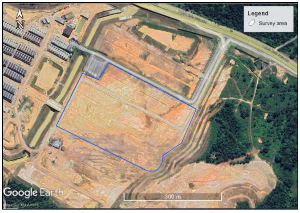
Location of survey area [18].
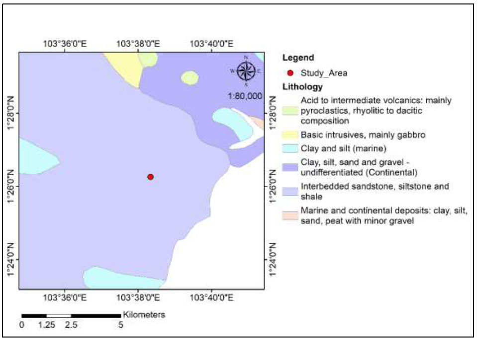
Regional geology of survey area [16].
2. SURVEY AREA AND GEOLOGY
The survey area was located at Iskandar Puteri, Johor, Malaysia, and covered 82,000 m2 area, which was cleared and flattened via cut and filled (Fig. 1). The area was located on sedimentary rock types: interbedded sandstone, siltstone, and shale of Triassic age, such as shown in Fig. (2) [16]. This tallies with the sandstone and siltstone outcrops found in the survey area (Fig. 3). It should be noted that geological information assists in the interpretation of geophysical data as structural complexities affect the strength of ground materials and seismic signals, which may lead to masking of the targeted layers in seismic processing and inaccurate depth computations of all layers beneath it [17].
3. MATERIALS AND METHODS
3.1. Seismic Refraction
This method provides insight into the strength of the ground subsurface materials based on their densities and modulus. It is one of the common geophysical methods used in engineering and environment applications to map bedrock [19]. The method correlates the travel time of the seismic waves (P-wave) with the density and elastic moduli of the earth material in its calculations.
Three seismic refraction survey lines (S1 – S3) were conducted where 24 channels of ABEM Terraloc Pro 2 seismograph were utilised together with 24 vertical geophones with 28Hz frequency each. Selection of geophone frequency plays a role in improving signal-to-noise ratio, as it can cut out unwanted noise, in addition to multiple shot point stacking during data acquisition [20]. A seismic source (18 lb sledgehammer) was used to generate strain energy by imposing it onto the ground to produce roughly 150 joules of energy. The energy propagates radially to produce direct, reflection, and refraction waves. At a particular distance, the waves reached the ground surface, were detected by geophones, and were recorded as a function of time by the seismograph, as depicted in Fig. (4).
All spreads used 5 m geophone spacing and seven (7) shot points. Five (5) shot points were located along the spread, while the other 2 were offset shots (before and beyond the spread) to enable deeper ground subsurface mapping. All survey lines had positive and negative 50 m offsets to increase penetration depth [21]. (Fig. 5) shows the seismic lines conducted. Two survey lines, S1 and S2, crossed each other at 54 m distance on SL1 and at 90 m distance on SL2. The lines were designed in a way that the two crossed lines (SL1 and SL2) would be used to correlate with each other, while the other survey line (SL3) was conducted to map and cover more area.
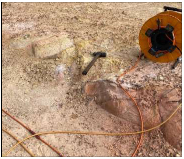
Sandstone outcrop found along the survey line.
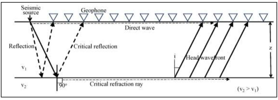
Seismic wave propagation from the shot point as a direct wave, reflection, and refraction rays [22].
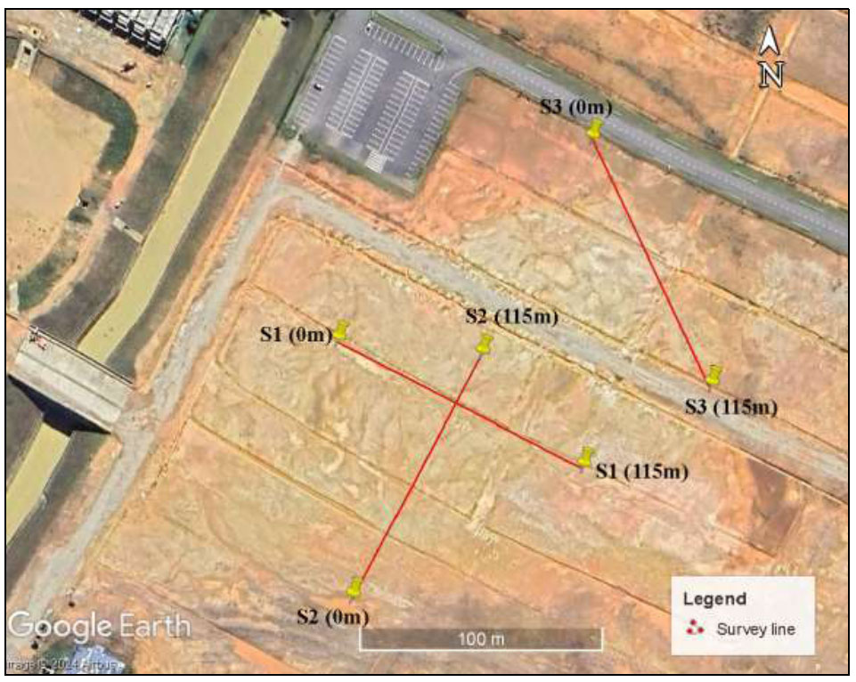
Seismic and electrical resistivity tomography (ERT) survey lines conducted [18].
The seismic refraction method has a limitation in detecting thin layers and hidden layers [17, 23]. A thin layer is defined as the minimum thickness of wavelength divided by two (λ/2), which is the maximum amplitude [24]. A layer is considered thin when its thickness is less than the dominant wavelength of the seismic wavefield that illuminates the bed. When the layer is too thin to produce first arrivals, the head wave arrives later in the time-distance graph, therefore making the thin layer (e.g., interbedded soils) a ‘blind zone’ or hidden layer that cannot be resolved [25].
The seismic refraction method is dependent on the basic principle of geological layering, where the density of earth material should increase with depth [24]. In the case where the upper layer (e.g., weathered rock Class II) has similar or greater velocities than the lower layer (e.g., weathered rock Class III), this will result in the lower layer (Class III) being masked/hidden by the upper layer (Class II) as the seismic waves cannot detect it and would cause depth calculations error, especially at greater depths [26, 27]. This is also called a hidden layer. It is vital to understand the concepts of thin and hidden layers for seismic refraction surveys, especially in structurally complex areas.
Data processing was divided into two stages;
3.1.1. Stage 1
The first arrivals of the P-waves were manually picked using SeisOptPicker for all spreads, and the first arrival times were plotted against the geophone distance (travel time graph) for each seismic shot point.
3.1.2. Stage 2
The data for first arrival times, shot positions, and geophone positions, including elevation, were imported into SeisOpt @2D v6.0 commercial software, which inverted the data to produce a P-waves velocity tomo- graphy profile. SeisOpt @2D is a refraction velocity optimization software that only requires the first-arrival picks and array geometry to derive velocity structural information, making the tool ideal in an area with limited information on subsurface velocity structure.
The velocity of seismic pulses depends on the densities and elastic moduli of the materials through which the waves propagate [28]. Therefore, the seismic velocity of a material is not fixed but varies depending on geology, fracturing, density, and elastic moduli [29]. Table 1 shows the seismic velocity values of common ground materials where their values were inferred during interpretation. To achieve an accurate interpretation, a comprehensive analysis was executed using seismic refraction results, geology, and neighbouring information.
| Material | Seismic Velocity (m/s) | |
|---|---|---|
| Igneous / Metamorphic | Granite | 4,000 – 5,800 |
| Weathered granite | 1,000 – 4,000 | |
| Basalt | 5,400 – 6,400 | |
| Sedimentary rock | Sandstone | 1,830 – 3,970 |
| Shale | 2,750 – 4,270 | |
| Limestone | 2,140 – 6,100 | |
| Unconsolidated sediment | Clay | 915 – 2,750 |
| Alluvium | 500 – 2,000 | |
| Sand | 200 – 2,000 | |
| Groundwater | Fresh water | 1,430 – 1,680 |
| Salt water | 1,460 – 1,530 | |
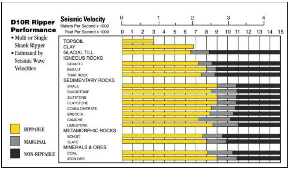
Rippability prediction based on seismic velocity chart of bulldozer D10R of Caterpillar [32].
3.2. Ground Rippability
Ground rippability for the survey area was determined by using the guideline on the correlation between the values of P-wave velocity (Vp) and the Caterpillar D10R rippability chart shown in Fig. (6) produced by Caterpillar Incorporation [32].
3.3. Weathering Grade
Due to the lack of borehole records in the study area, weathering grades of the ground were estimated by referring to the correlation between seismic Vp values and weathering grades from a journal paper published by a previous study [14] with a similar geological setting (sedimentary rock). Referring to Table 2, the seismic profiles of S1 – S3 were classified into five groups of weathering grades: VI, VI-V, V-IV, IV-III-II, and III-II-I.
4. RESULTS AND DISCUSSION
The P-waves refraction first arrivals for all seismic lines S1, S2, and S3 were picked and plotted in distance-travel time graphs as shown in Fig. (7). To process the seismic profiles, seismic refraction tomography was conducted instead of the conventional processing method, Generalised Reciprocal Method (GRM). GRM is good in mapping laterally by assuming the ground subsurface is in layered media with increasing seismic velocities [33, 34]. However, the ground subsurface produced from GRM often contradicts observed ground characteristics due to its limitation in detecting heterogeneity, lateral discontinuities, and gradients [35]. Seismic refraction tomography is superior to GRM as it is capable of resolving both vertical and lateral velocity changes and velocity gradients [7, 36, 37]. Hence, this study applied seismic refraction tomography in processing seismic results to produce seismic velocity profiles, as shown in Fig. (8).
| Velocity (m/s) | Ground Material Description | Weathering Grade |
|---|---|---|
| < 300 | Subsurface soil and much loosened ground. Very dry condition. | VI |
| 300 – 800 | Gravelly to clayey silty sand. | VI – V |
| 800 – 1,800 | Gravelly to clayey, silty sand; completely weathered to highly weathered with evidence of highly fractured rock. | V – IV |
| 1,800 – 2,400 | Highly weathered to Moderately weathered rock. | IV – III – II |
| > 2,400 | Moderately weathered to slightly weathered zone and fresh rock. | III – II – I |
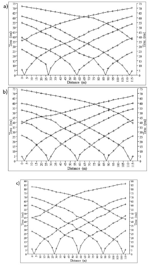
Distance-travel time graphs for seismic lines a) S1, b) S2, and c) S3.
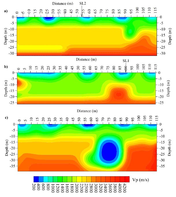
Seismic refraction profile for seismic lines a) S1, b) S2, and c) S3.
The results show that the ground subsurface in the study area had a velocity of P-waves (Vp) that ranged between 200 – 4,400 m/s with a maximum penetration depth of 26.3 – 39.4 m, as shown in Table 3. The difference in penetration depth between each profile is due to the density and velocity of the ground subsurface beneath the survey lines, where the low-velocity layer in S2 (Vp< 2,000 m/s) is approximately twice thicker than present in S1 and S3. This shows that less competent ground mass would lead to shallower penetration depth, as stated by Alsamarraie [38] and Imani et al. [5], due to seismic signal attenuation. Obermann et al. [39] also stated that the depth sensitivity of seismic waves is affected by the degree of ground heterogeneity and velocity changes, which explains the difference in penetration depth between survey lines S1, S2, and S3.
At the intersection point between lines S1 and S2, the seismic values Vp are consistent in both profiles (54 m distance on S1 and 90 m distance on S2), which signifies good and reliable first arrival pickings. Considering sandstone outcrops can be found at some parts of the survey lines, as in Fig. (3), by referring to Table 1, it can be surmised that the seismic profiles have penetrated bedrock. This is proven by the presence of Vp values that are greater than 1,830 m/s (minimum sandstone value) in all survey lines.
| Line | Vp (m/s) | Depth (m) |
|---|---|---|
| S1 | 200 - 4400 | 31.9 |
| S2 | 200 - 4400 | 26.3 |
| S3 | 200 - 4400 | 39.4 |
From the outcrop on site, certain parts of the seismic survey lines cut across the sandstone layer. Therefore, the ground subsurface is classified based on its rippability using the correlation between P-wave velocity values (Vp) of sandstone and the Caterpillar D10R rippability chart. The correlation produces a three-layer case of the ground, which are rippable (Vp of <2,500 m/s), marginal (Vp of 2,500 – 3,200 m/s), and non-rippable (Vp of >3,200 m/s), as shown in Table 4 and (Fig. 9). The rippable layer is thinnest along line S3, which is approximately 15m from the surface, followed by lines S1 and S2. Breaks in the continuous layering seen in lines S1 and S3 are due to the presence of fracture, which causes a decrease in the density of rock mass [40]. This fracture causes a discontinuity in the rock mass, which is a common characteristic of sedimentary rock and affects the change in seismic waves’ travelling velocity via dispersion, in addition to geometric and intrinsic attenuation factors of the fracture structures [41, 42]. This consequently results in a decrease of Vp values in the fracture zone, which is sandwiched between high Vp values. Meanwhile, a boulder can be detected in line S2 at a distance of 0 m, having a higher seismic Vp value than the surroundings [43]. This proves that the more weathered a rock mass is, the lower its velocity. Therefore, layer 1 with the lowest Vp is the easiest to excavate, while layer 3 with the highest Vp is not excavatable using Caterpillar bulldozer D10R due to its solid rock mass.
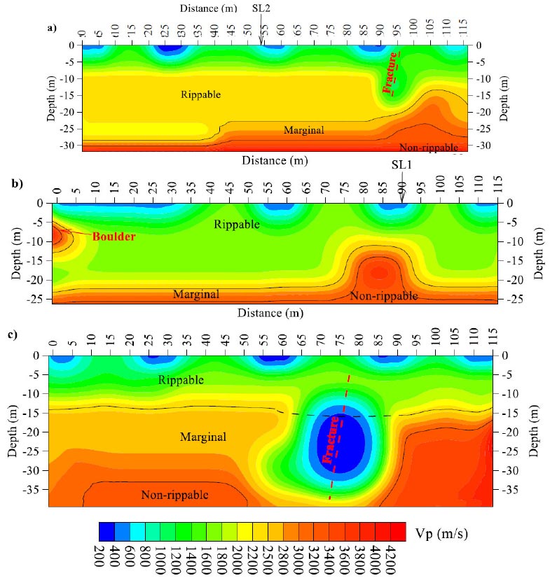
Rippability of the ground based on correlated seismic refraction velocity (Vp) values for lines a) S1, b) S2, and c) S3.
| Vp (m/s) | Layer | Rippability |
|---|---|---|
| <2,500 | 1 | Rippable |
| 2,500 – 3,200 | 2 | Marginal |
| >3,200 | 3 | Non-rippable |
Based on Table 2 by Ismail et al. [14], weathering grades of the ground subsurface for all lines were determined as shown in Fig. (10), where the weathering grade decreases with depth. This tallies with the common geological profile where the ground becomes denser with depth due to compaction and lower soil strength [29, 44], while rock mass becomes less fractured with increasing depth [38, 45, 46]. Weathering grades of moderate to slightly weathered zone and fresh rock (III-II-I) were shallower in survey lines S1 and S3, while the weathering grades occurred much deeper in S2.
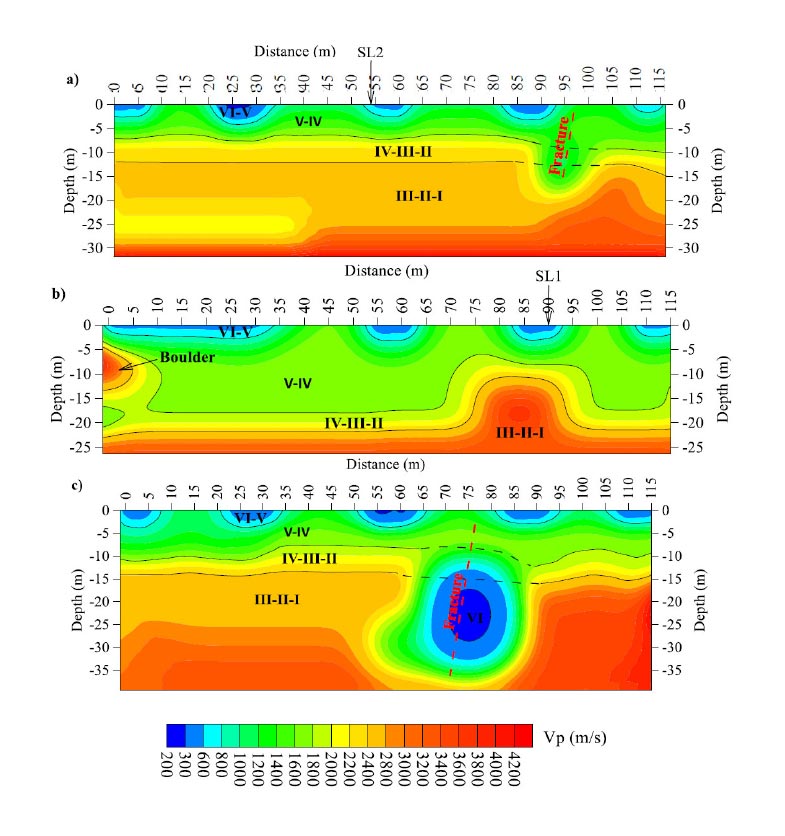
Weathering grade of the ground based on correlated seismic refraction velocity (Vp) values for lines a) S1, b) S2, and c) S3.
CONCLUSION
A seismic refraction survey was conducted at Iskandar Puteri (Johor) to investigate the rippability and weathering grades of the ground in a sedimentary rock geological setting (interbedded sandstone, siltstone, and shale). Based on seismic Vp values and the Caterpillar D-10R rippability chart, the study classified the ground into three layers: rippable, marginal, and non-rippable layers. As the study area does not have any borehole records, weathering grades of the ground were determined based on a similar case study in a published journal. From the seismic Vp values, the ground was successfully classified into five groups of weathering grades: VI, VI-V, V-IV, IV-III-II, and III-II-I.
AUTHORS’ CONTRIBUTION
It is hereby acknowledged that all authors have accepted responsibility for the manuscript's content and consented to its submission. They have meticulously reviewed all results and unanimously approved the final version of the manuscript.